Jackson et al. (2023). “Metrics for Optimizing Searches for Tidally Decaying Exoplanets.” AJ, 166, 4.
Brian’s publications
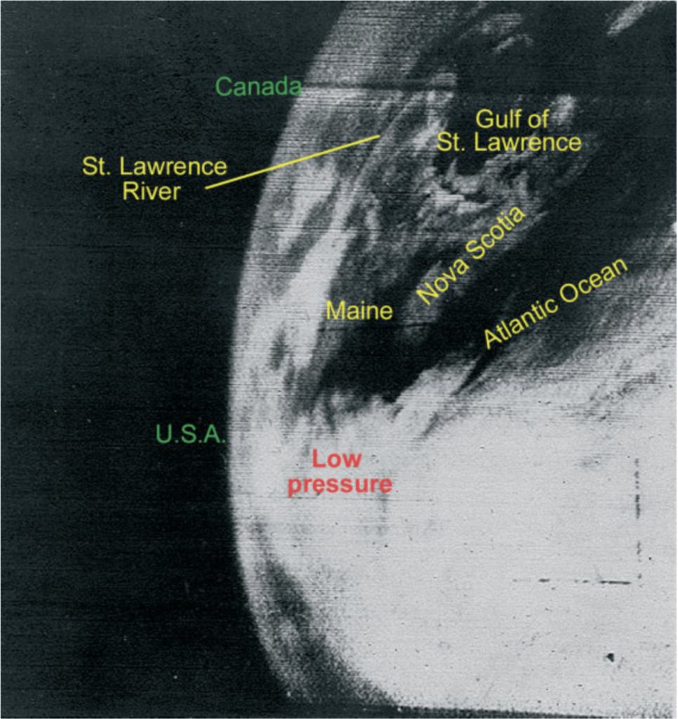
On April 1, 1960, NASA took the first weather satellite picture onboard TIROS-1, the Television and Infra-Red Observation Satellite.
In spite of its name, TIROS-1 could only collect images in visible wavelengths, but over its nearly two-month mission, it collected more than 20,000 images of weather systems from an altitude of 700 km, launching the ancient science of meteorology into the space age.
Since those early successes, scientists have found a bewildering variety of weather patterns across the solar system.
For instance, on Venus, a stratospheric jet stream jet stream on steroids herds clouds around the planet every four days, even though it takes almost a year (243 days) for the solid body of Venus to rotate once on its axis (the Earth only takes 24 hours).
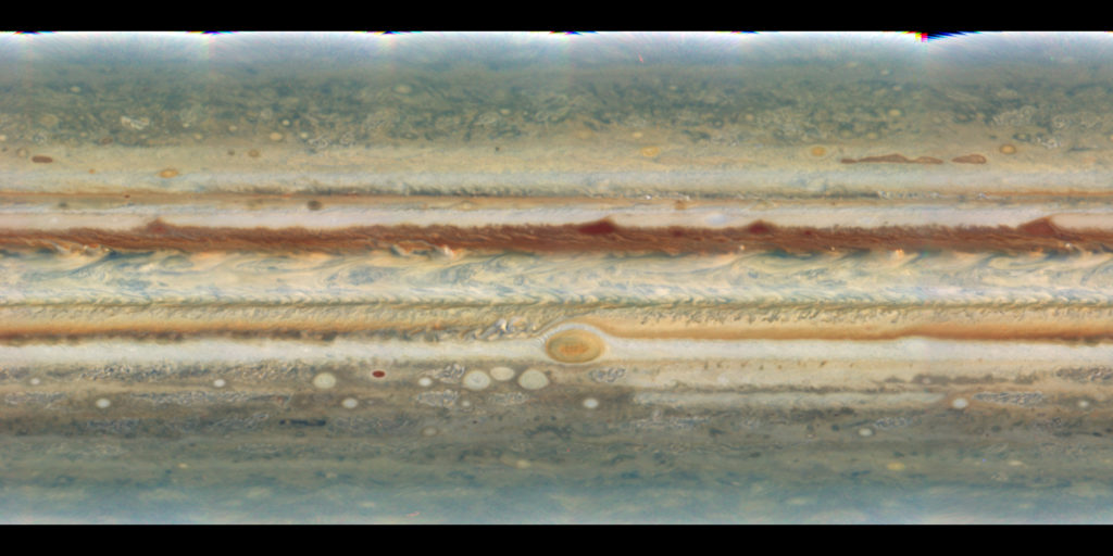
A much faster rotator, Jupiter also exhibits jet streams, and, as seems fitting for the largest planet in the solar system, the jet streams are so massive they induce a measurable gravitational signature recently detected by NASA’s Juno mission currently orbiting the king of planets.
We’ve even managed to extend our meteorological studies beyond the solar system. In 2007, Heather Knutson and colleagues used soon-to-be-decommissioned Spitzer Space Telescope to create a low-res map of the atmosphere of the hot gas giant HD189733b in infrared wavelengths.
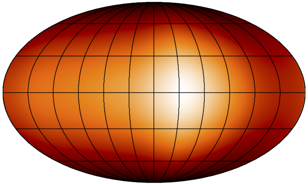
Unlike planets in our own solar system, we can’t directly image HD189733b — it’s too far away. So Knutson and colleagues used a trick to map HD189733b. Since the planet orbits very close to its host star (it circles the star once every 2 days), tidal interaction with the star has probably locked the planet’s dayside to always face the star and the nightside to always face away (reminiscent of the Moon’s rotation).
Knutson and colleagues created their map by simply watching HD189 circle its host star, and as the bright dayside rotated in and out of view, they watched as the amount of light from the planet went up and down. This up and down, called a planetary phase curve, allowed them to decipher which regions on the planet were brighter than others.
And what they found was a little surprising. Even though the planet’s dayside always points toward the star, the hottest place in the planet’s atmosphere wasn’t the place that receives the most sunlight (the “sub-stellar point“) — it was about 3,500 km to the east. Why?
Since HD189 is tidally locked, the dayside is MUCH hotter than the nightside, and this very large temperature contrast drives a super-rotating jet. This jet carries gas through the sub-stellar point at thousands of miles per hour, and by the time the gas has a chance to heat up, it’s already thousands of miles downwind.
But even though jet streams like this can be permanent features in a planet’s atmosphere, they are highly dynamic. For instance, the periodic appearance over the midwestern US of polar vortices result from meanders in the Earth’s jet stream. Since jet streams on hot Jupiters are driven by thousand-mile-an-hour winds, we might expect even more dramatic variability.
Cued by these expectations of jumpy jet streams, our research group studied the planet Kepler-76b, a Jupiter-sized planet zipping around its host star every 1.5 days. The planet is so close to its star that it’s as hot (2200 K or 3500 degrees F) as some low-mass stars.
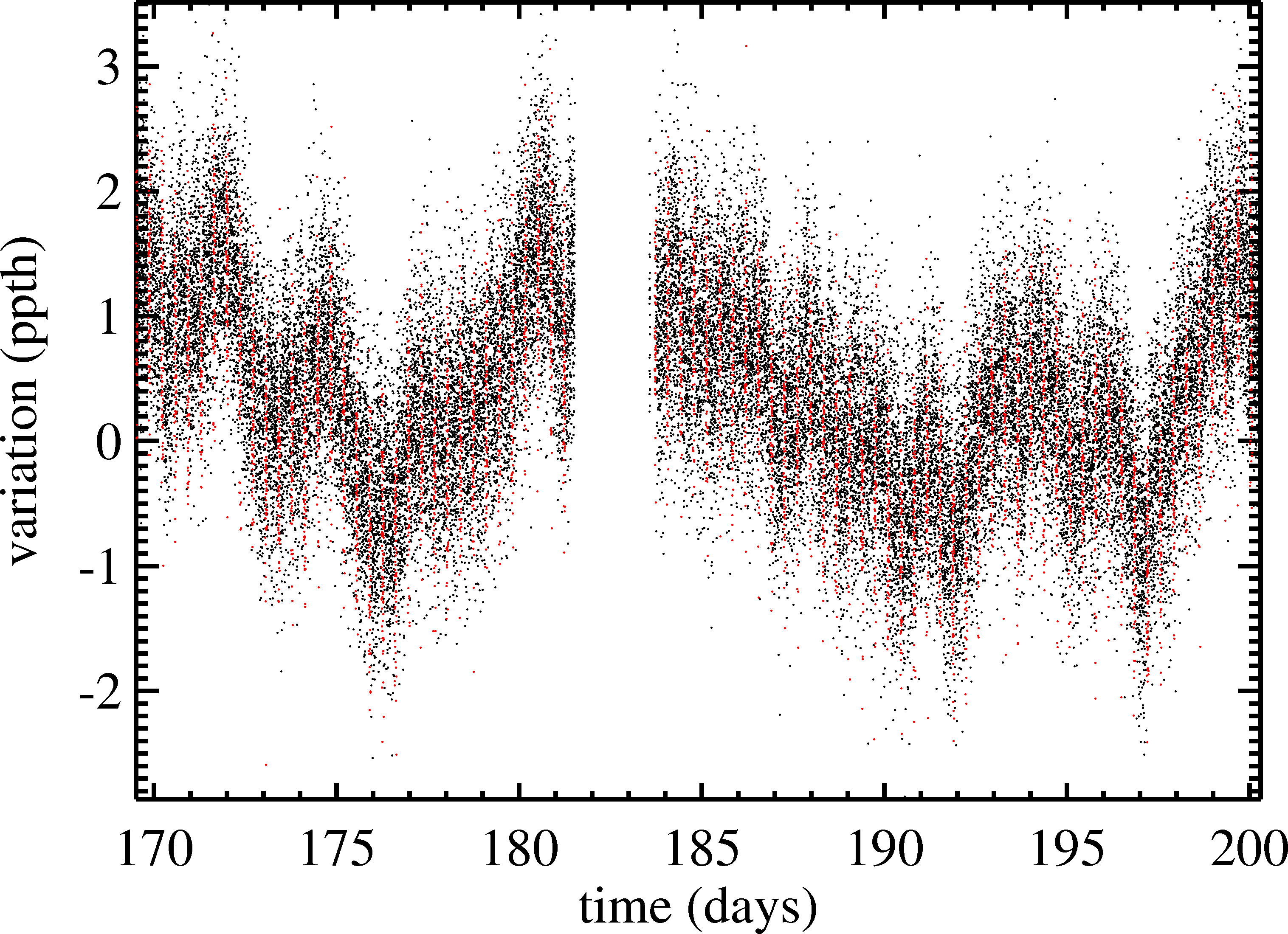
We analyzed phase curve observations of Kepler-76b collected several years ago by the Kepler Mission, which stared at the planetary system for more than 3 years, which gave us a lot of data to work with.
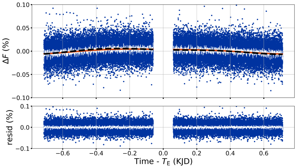
The blue dots in the figure above shows the subtle up-and-down phase curve for Kepler-76b. In our analysis, we found that up-and-down went up a lot during some orbits and much less on others. All told, these variations amounted to changes in the planet’s dayside temperature of hundreds of degrees.
What’s causing this variability? The short answer is we don’t know. But we have some guesses. Previous work has shown that, although Kepler-76b’s dayside is much too hot for clouds (they quickly vaporize), the super-rotation can transport clouds from the nightside.
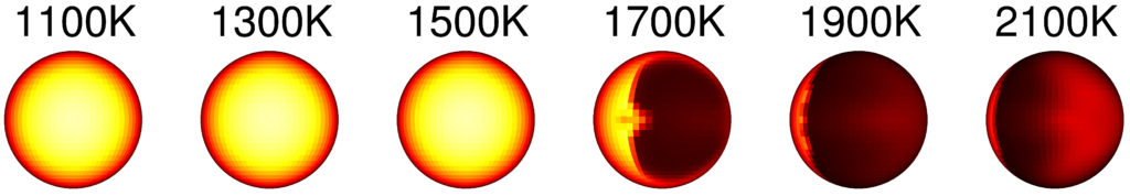
We expect that when Kepler-76b’s dayside gets a little cloudy, it will get a little brighter, meaning the phase curve will have more up and down. But since the dayside clouds would now be reflecting more sunlight, that means the dayside will get a little cooler (like on a cloudy day on Earth).
Since the windspeed of the jet stream depends on the temperature contrast between the day and nightsides, a cooler dayside presumably means a weaker jet. The clouds transported to the dayside then evaporate, and the weaker jet cannot bring clouds from the nightside quickly enough to resupply them. Thus, the clouds clear out, the dayside loses its cooling shroud and heats up, which strengthens the jet and starts the cycle all over again.
As in all things science, more studies are needed to decide whether this scenario actually plays out in the atmosphere of Kepler-76b and other hot Jupiter. But for now, studies like ours show that the same kinds of meteorological processes seen on the Earth from space 60 years ago can also be seen on worlds beyond our solar system.
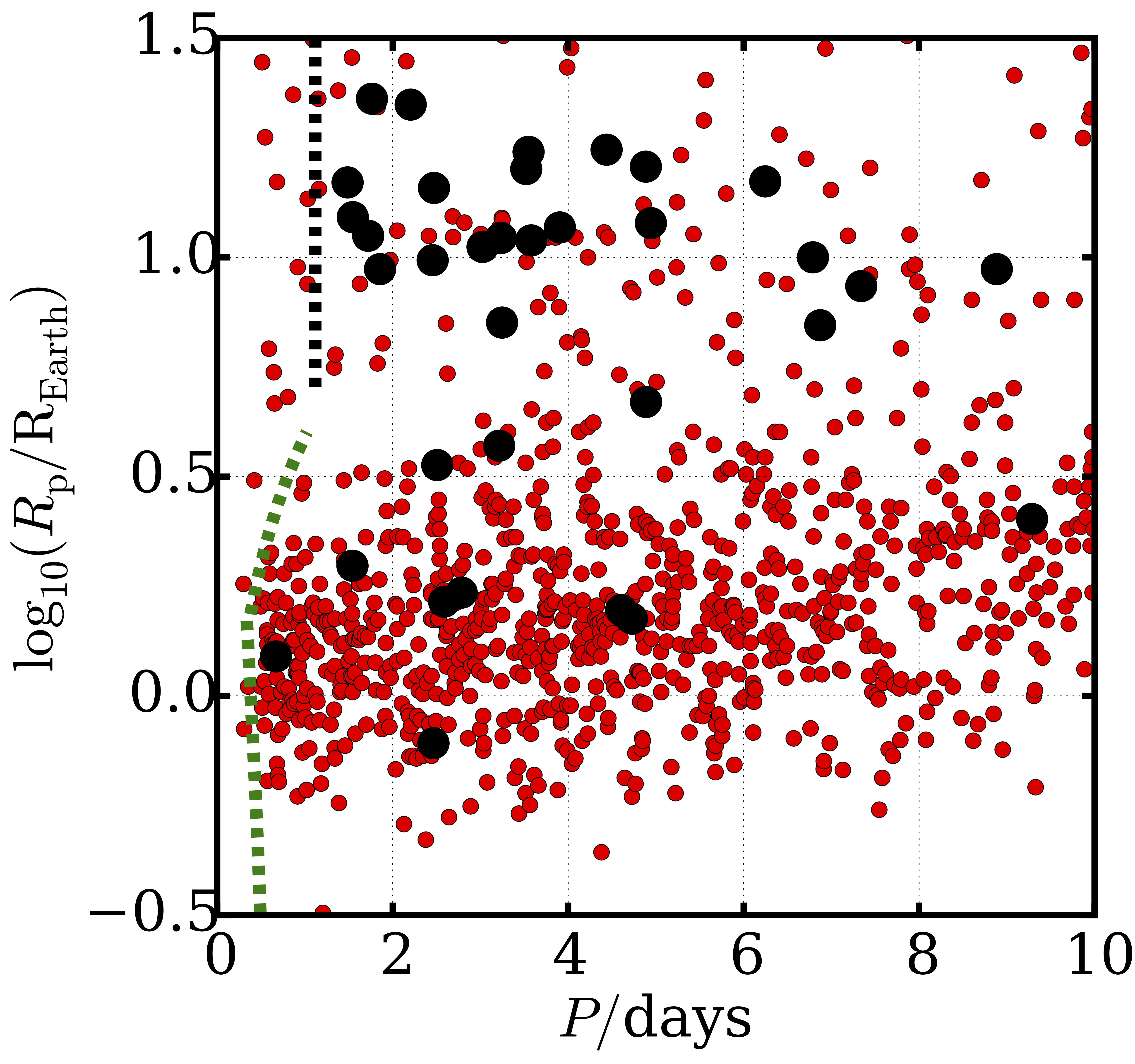
Planetary radii and orbital periods for planets (black circles) and planetary candidates (red circles) discovered by the Kepler mission. The dashed curves shows how close different planets can get to their host stars before they would be tidally disrupted. Taken from Jackson et al. (2016).
Exciting news – just today, my research group had another paper accepted for publication, so we’ve added one more tiny brick to the edifice of human knowledge.
This paper explored tidal disruption of gaseous exoplanets. Over the last few decades, astronomers have discovered thousands of planets outside of our solar system, so-called “exoplanets”.
Most of the planets do not resemble planets in our solar system, and owing to biases in the way we find the planets, many of them are big, gas balls like Jupiter but orbiting much closer to their host stars than planets in our solar system – these planets are called “hot Jupiters“. The figure at left shows how close some of these planets are to their host stars.
Many of these hot Jupiters are doomed to spiral in toward their host stars, and when they get too close, the star’s gravity can rip them apart in a process called “tidal disruption“.
In our recent paper, we studied that process to try to understand how close a planet can get before it’s ripped apart and what might happen as it’s being ripped apart. The upshot of our study is that planets might get ripped apart a little farther from their stars than is often assumed BUT that ripping-apart process might proceed fairly slowly, over billions of years.
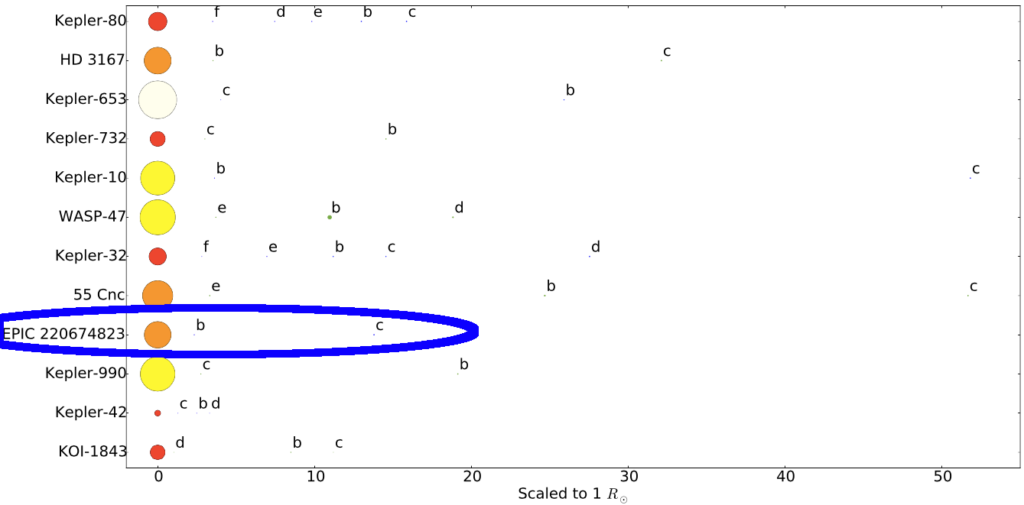
Twelve multi-planet systems where the innermost member is very close to the host star, that is, has an orbital period less than 1 day. From Adams et al. (2016).
Big research news today: our research group SuPerPiG, led by the inimitable Dr. Elisabeth Adams, announced the discovery of two new planets, EPIC 220674823 b and c.
Using data from the K2 Mission, we found these planets by looking for the shadows of the planets as they passed in front of their host stars, a planet-hunting technique known as the transit method.
These new planets are very different from planets in our solar system in several surprising ways.
First, they’re both bigger than Earth but smaller than Neptune – planet b is 50% larger, and planet c is 2.5 times larger. They inhabit a strange nether-region of planets where they’re known as super-Earths or sub-Neptunes, planets somewhere between Earth and Neptune. The reason there’s no specific name for such planets is because astronomers don’t understand this new class of planet at all.
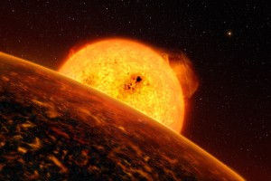
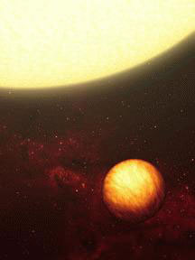
An artist’s conception of CoRoT-7 b, another ultra-short-period planet.
Second, both planets are MUCH closer to their Sun than the planets in our solar system. In fact, planet b is so close to its sun that it takes less time to orbit (14 hours) than all the playtime it took the Cubs to go from 3 games down to tying up the World Series. By comparison, planet c circles at the glacial pace of once every 13 days.
Another thing that’s interesting about our planets: they’re yet another system of with an ultra-short-period planet (USP) in which there is more than one planet, i.e. a multi-planet system. In fact, as we argue in our paper, most of the known systems with ultra-short-period planets are probably multi-planet systems and that fact might help explain the origin of these chthonic planets.
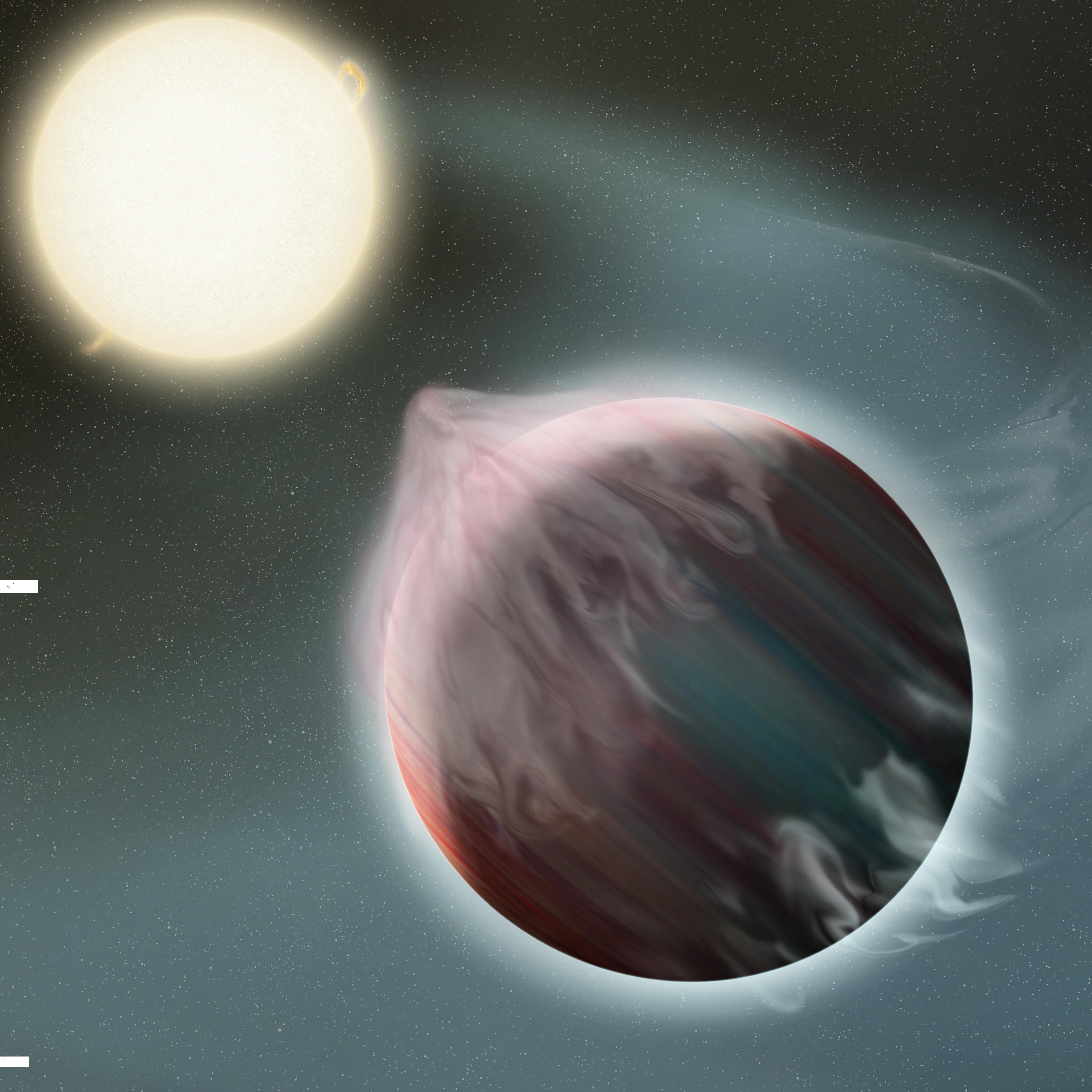
Artist’s conception of tidal disruption of a gas giant planet.
In the last few decades, astronomers have discovered thousands of extrasolar planets, and there seems to be, on average, one planet for every star in the galaxy. Some of the planets are like those in our solar system, but many are not.
In fact, there’s a huge number of gas giant planets, like Jupiter, but on such short-period orbits they are nearly skimming the surfaces of their stars. These hot Jupiters are actually so close to their host stars, they are in danger of being torn apart by the stars’ gravity.
In a study just accepted for publication, my research group investigated what happens to a giant planet when it is ripped apart. We found that, over a few billion years, these planets can lose their entire atmospheres, leaving behind the little rocky core deep in the planet’s interior.
It also turns out that, as the planets lose their atmospheres, they can also get pushed out away from the star, and our study found that how much the planet gets pushed out depends pretty sensitively on the size of the rocky core.
That’s pretty neat because it means we can compare the masses and orbits of known rocky exoplanets to what we would expect if those little planets were actually the fossil cores of bigger gas giants that had their atmospheres ripped off.
The figure below shows how the current orbital periods of known planets P compares to what we’d expect if they were fossil cores, P_(Roche, max). In some cases, there’s a decent match, but in lots of cases, there’s not. So we’ve still got some work to do.
UPDATE (2016 Mar 24): The paper is now available for free on astro-ph.
The Astrophysical Journal published today a paper by my colleagues and myself investigating in detail a way to look for moons around transiting exoplanets.
The discoveries of thousands of planets and planetary candidates over the last few decades has motivated a parallel effort to find exomoons. In addition to providing a base of operations for the Empire, exomoons might actually be a better place to find extrasolar life than exoplanets in some ways.
This technique for finding exomoons, called the Orbital Sampling Effect, was developed by René Heller and involves looking for the subtle signature of a moon’s shadow alongside the shadow of its transiting planet host, as depicted in the image below.
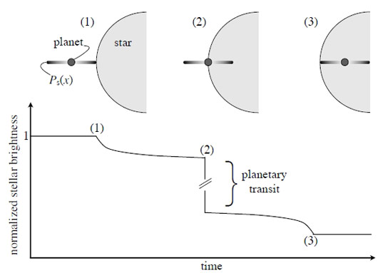
The dark cloud shown around the planet represents the exomoon’s shadow, averaged over several orbits. At epoch (1), a satellite transits just before the planet. At epoch (2), the planet’s transit begins, inducing a large dip in the measured stellar brightness. At epoch (3), the satellite modifies the planet’s transit light curve slightly but measurably.
This simple technique has advantages over alternative exomoon searches in that it doesn’t require significant computational resources to implement. It can also use data already available from the Kepler and K2 missions. However, on its own, the technique can’t provide a moon’s mass, only its size, and it requires many transits of the host planet to find the moon’s quite subtle transit signature.
No exomoon has been found yet in spite of tremendous efforts to find them, so the search continues.
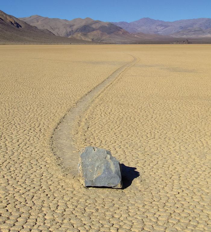 “Tucked away in California’s Death Valley National Park, the flat basin known as Racetrack Playa is littered with stones that seem to migrate across the landscape. But how do they do it? Brian Jackson describes how he and collaborators Ralph Lorenz and Richard Norris solved a long-standing mystery.” http://physicsworld.com/cws/article/indepth/2015/jul/02/the-restless-rocks-of-racetrack-playa
Thanks to Ralph and Dick for their help with this article. It was a lot of fun to write.
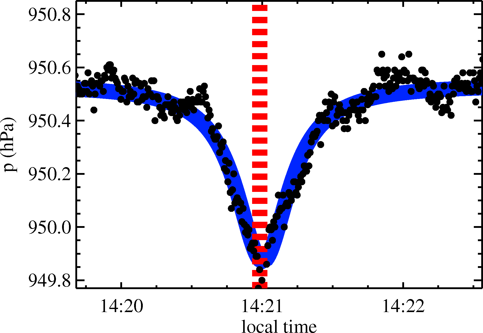
Pressure variations (in hectoPascal, hPa) vs. local time for one dust devil pressure dip. The blue curve shows our model fit.
Dust devils occur in arid climates on the Earth and ubiquitously on Mars. Martian dust devils have been studied with orbiting and landed spacecraft, while most studies of terrestrial dust devils have involved manned monitoring of field sites, which can be costly both in time and personnel. As an alternative approach, my colleague Ralph Lorenz and I performed a multi-year in-situ survey of terrestrial dust devils using pressure loggers deployed at El Dorado Playa in Nevada, USA, a site known for dust devil activity.
When a dust devil passed over our pressure sensors, it appeared as a pressure dip in the time series, as illustrated in the figure. By modeling these signals, we learned a lot of about dust devils. For instance, in spite of expectations, we found signals that looked a lot like dust devils that occurred at night and even in the winter. So do dust devils happen year-round, day and night? More work will help us figure it out.
Our paper on this study will appear soon in the Journal of Geophysical Research Planets.
Synthetic data for the new pointing capabilities of Kepler, showing the expected brightness variations for a planet hosting a star that transits (i.e., the planet passes in front of the star, blocking out some of the light). The red points show when the planet is transiting.
Recently, the Kepler mission announced that two reaction wheels on the spacecraft have failed, and so the telescope won’t be able to point as accurately as before. As a result, data from the telescope will suffer from large instrumental variations (see figure at right), and so it will be difficult to detect Earth-like planets. However, the telescope may be able to detect other kinds of planets and study other astronomical phenomena.
In response to a request from Kepler for new ideas of what to do with the telescope, I wrote about an idea to search for very short-period (less than 1 day) planets. A re-purposed Kepler mission could continue the search for nearly Earth-sized planets in very short-period orbits. Our recent work revealed more than a dozen such planetary candidates, and a more complete and focused survey is likely to reveal more.
