data science

All posts tagged data science

svmregression

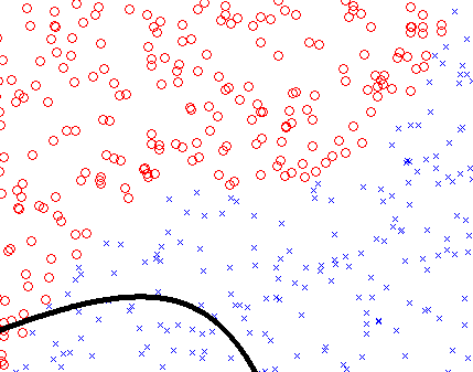
Animation showing how a machine-learning algorithm decides where lies the boundary between two classes of objects.

Third day of the DPS Meeting was full of fascinating talks about the orbital architectures of exoplanet systems.

One that caught my attention was Dan Tamayo‘s talk on using machine-learning to classify the stability of a planetary system.

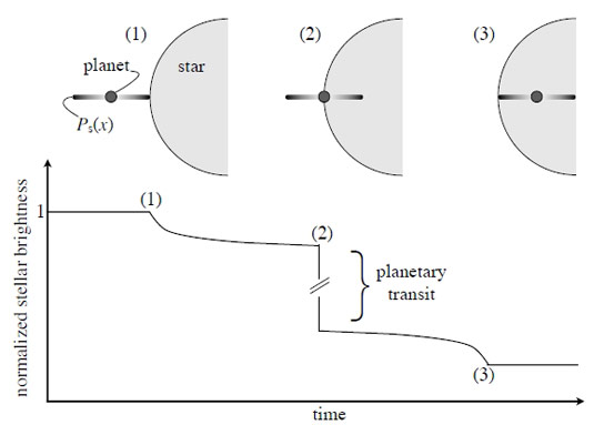
As astronomers have discovered more potential planetary systems, it’s becoming more time-consuming to decide whether what we see are actually planets or some other thing that has fooled us into thinking they’re planets.

When astronomers find what they think might be a planetary system, one of the first things they check is whether the putative planetary system is actually stable — that is, whether the gravitational tugs among the putative planets would cause the objects to crash into one another or be thrown out of the system.

Since most of the planetary systems we find are probably billions of years, astronomers expect that real planetary systems are stable for billions of years, so if the system we’re looking out turns out to be unstable on short timescales (less than billions of years), we usually decide that it’s not really a planetary system (or that we mis-estimated the planetary parameters).

Unfortunately, doing this check usually requires running big, complicated computer codes, called N-body simulations (“N” for the number of planets or bodies in the system) for hundreds or thousands of computer-hours. That can be a problem if you’ve got planetary candidates flooding in, as with the Kepler or upcoming TESS missions.

Tamayo wanted to try a different approach: what if the same machine-learning techniques that allow Google or Facebook to decide whether someone is likely to buy an iPhone could be used to more quickly decide whether a putative planetary system was stable

So Tamayo created many, many synthetic planetary systems, some stable, some not, and had his machine-learning algorithm sort through them. According to Tamayo, his scheme was able to pick up on subtle features that helped distinguish stable systems from unstable ones with very high accuracy in a fraction of the time it would take to run an N-body simulation.

aaeaaqaaaaaaaamaaaaajdjmowm5yzjjlwjhzgitnge4ys05ogi3lwu4mdjmmmi4zgexyq
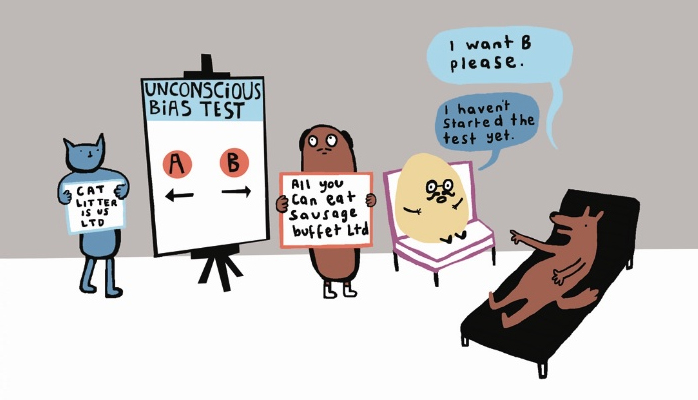
I also attended an eye-opening talk from Patricia Knezek of NSF about unconscious biases and their effects in astronomy and planetary science. Knezek explained that several studies have shown how these biases cause everyone to draw unconscious conclusions about someone based on very cursory information, such as their first name, race, gender, etc.

For instance, one study showed that the same application for a faculty position did much better if the applicant’s first name was “Brian” instead of “Karen”, even when women were evaluating the application.

Fortunately, these same studies have shown several ways to mitigate the effects of these biases, and being aware of them is a big first step.

UPDATE (2016 Mar 24): The paper is now available for free on astro-ph.

The Astrophysical Journal published today a paper by my colleagues and myself investigating in detail a way to look for moons around transiting exoplanets.

The discoveries of thousands of planets and planetary candidates over the last few decades has motivated a parallel effort to find exomoons. In addition to providing a base of operations for the Empire, exomoons might actually be a better place to find extrasolar life than exoplanets in some ways.

This technique for finding exomoons, called the Orbital Sampling Effect, was developed by René Heller and involves looking for the subtle signature of a moon’s shadow alongside the shadow of its transiting planet host, as depicted in the image below.

At epoch (1), a satellite’s transits just before the planet. At epoch (2), the planet's transit begins, inducing a large dip the measured stellar brightness. At epoch (3), the satellite modifies the planet's transit light curve slightly but measurably.

The dark cloud shown around the planet represents the exomoon’s shadow, averaged over several orbits. At epoch (1), a satellite transits just before the planet. At epoch (2), the planet’s transit begins, inducing a large dip in the measured stellar brightness. At epoch (3), the satellite modifies the planet’s transit light curve slightly but measurably.

This simple technique has advantages over alternative exomoon searches in that it doesn’t require significant computational resources to implement. It can also use data already available from the Kepler and K2 missions. However, on its own, the technique can’t provide a moon’s mass, only its size, and it requires many transits of the host planet to find the moon’s quite subtle transit signature.

No exomoon has been found yet in spite of tremendous efforts to find them, so the search continues.


OCR OC-gain

My PHYS341 students were interested to see how the OCR routine processed their attendance sheet, so I applied it, as shown below.

IMG_3707_orig-scannedThe left panel shows the original, the right the transformed version. The routine did a reasonable job of un-distorting the page (although it wasn’t too bad to begin with).

And here’s what the routine returns as text:

zolto J:)o<-&\
Qfick ${‘bt\L . .
1ZWrW(\ DQVCS
Onras Tkomag
Jam; I-Em!
De»-UV1, ?I‘L\M‘ovV\QJ3€,v'
Ia./I B,a,C/IHMC .
V.o\3 \3<<I°\Ser&eck
jengifcr Brigga
}VK°'('3E\V1c-rad LULAA
Mby Ouersfreci’ '
Tm (jivws ‘
gj)/VIOI/I  ‘
$030-4 “10u\J ‘
{NC /I/1a.V,,,,',q '
O”AKe So/ares
Skwm \<reyc}~e '

…not great.

I’m not totally sure what went wrong. Maybe I should have them write their student numbers instead.

UPDATE: 2016 Feb 5

Here’s another go with a different attendance sheet. Not much better.

IMG_3784_scanned

I‘/\0,;/{¢r\(~  VETEK BROWN
E ? RICH/W} WLMC/(
“$2114!/~, lZoAr.‘%o Pratt.‘
D“""‘ 8'3"’ ' g/"It; /Vlar,//'/1
 Lolpef‘
kpdkl/n\‘f 2011/(IE
ANN <5©<J\M) Vfxit %'L0V\€z &}"-:5 _)_La/\/MAS _ Karm I>q'v‘-5
\Tou—o0l Hand _
'Dz\m/L ?\c\n'ksvvuu‘ev*
Ian I3/¢«'-Ckfia/If ¢
94% \5<<k*?l6<:x\.cLl¢ Jennifer BH995 N\o+‘\'V\c\.6 Luv\0\ . \/\0\\)y 0\,ers+reeJr ’\".m C"\\/Ens _ 51 m cm E 1: Y Jason May A ZPM > M
PIJW1 figu//
jam 5°0W'/J
34681 \4'€y¢}~¢>/

IMG_2366Final day of the IAU meeting  general assembly found me in talks about transit-timing variations, tidal interactions, and planets in binary star systems.

The first session focused on the impressive results from transit-timing variation (TTV) studies. Since detecting and modeling TTVs is very data-intensive, the talks explored the data science aspects of TTV analysis. Ben Montet‘s talk, for example, looked at how hard it can be to detect transits in the first place, much less measure their period variations. To estimate uncertainties on their variations, he advocated using importance sampling and generating thoroughly explored prior distributions.

The next session looked at tidal interactions and planets in binary star systems. Smadar Naoz talked about her work on Kozai oscillations and how she showed that Kozai had made some fairly specific assumptions that limited his famous dynamical analysis in important ways. Her improved analysis shows that, contrary to the original results, the Kozai mechanism can actually produce planets on retrograde orbits and so can help explain the growing number of such retrograde planets.

I also spoke in the second session about Roche lobe overflow in short-period gaseous exoplanets, and I’ve posted my presentation below.

So, all in all, a really brilliant conferences in an inspiring locale. Mahalo, Hawaii.

Tidal Decay and Disruption of Gaseous Exoplanets

As part of a project, I’m trying to learn how to do motion capture on videos. Fortunately, there’s Python support for the OpenCV computer vision library.

I adapted some motion capture code I found online that uses the Shi-Tomasi Corner Detector scheme to find good features to track — regions in a grayscale video frame that have large derivatives in two orthogonal directions.

Then the code estimates the optical flow using the Lucas-Kanade method, which applies a least-squares fit to solve for the two-dimensional velocity vector of the corner features.

As a test case, I used a video of Alice singing the “Ito Maki Maki” song.

The shiny tracks in the video show the best-fit model. Interestingly, the corner detection scheme chooses to follow the glints in her eyes and on her lip. The motion tracker does a good job following the glints until she blinks and swings her arm across her face.

The code I used is posted below.

import numpy as np
import cv2
cap = cv2.VideoCapture('IMG_0986.mov')
size = (int(cap.get(cv2.cv.CV_CAP_PROP_FRAME_WIDTH)),
int(cap.get(cv2.cv.CV_CAP_PROP_FRAME_HEIGHT)))

# params for ShiTomasi corner detection
feature_params = dict( maxCorners = 100,
qualityLevel = 0.3,
minDistance = 7,
blockSize = 7 )

# Parameters for lucas kanade optical flow
lk_params = dict( winSize = (15,15),
maxLevel = 2,
criteria = (cv2.TERM_CRITERIA_EPS | cv2.TERM_CRITERIA_COUNT, 10, 0.03))

# Create some random colors
color = np.random.randint(0,255,(100,3))

# Take first frame and find corners in it
ret, frame = cap.read()
old_gray = cv2.cvtColor(frame, cv2.COLOR_BGR2GRAY)
p0 = cv2.goodFeaturesToTrack(old_gray, mask = None, **feature_params)

# Create a mask image for drawing purposes
mask = np.zeros_like(frame)

images = list()

height , width , layers = frame.shape

fourcc = cv2.cv.CV_FOURCC('m', 'p', '4', 'v')
video = cv2.VideoWriter()
success = video.open('Alice_singing.mp4v', fourcc, 15.0, size, True)

ret = True
while(ret):
  print(ret)

  frame_gray = cv2.cvtColor(frame, cv2.COLOR_BGR2GRAY)

# calculate optical flow
  p1, st, err = cv2.calcOpticalFlowPyrLK(old_gray, frame_gray, p0, None, **lk_params)

# Select good points
  good_new = p1[st==1]
  good_old = p0[st==1]

# draw the tracks
  for i,(new,old) in enumerate(zip(good_new,good_old)):
    a,b = new.ravel()
    c,d = old.ravel()
    cv2.line(mask, (a,b),(c,d), color[i].tolist(), 2)
    cv2.circle(frame,(a,b),5,color[i].tolist(),-1)

  img = cv2.add(frame,mask)

  video.write(img)
  ret,frame = cap.read()

# Now update the previous frame and previous points
  old_gray = frame_gray.copy()
  p0 = good_new.reshape(-1,1,2)

cap.release()
video.release()
cv2.destroyAllWindows()

With the help of physics major Jared Hand, we’ve started a weekly meeting group here in physics to discuss scientific computing — the Boise State SciComp Workshomp.

The meetings take place in the physics building, room MP408, and will focus on the nitty gritty of scientific computing — how to install and run various codes and packages.

We’ve started a github repository for the group: https://github.com/decaelus/BoiseState_SciComp_Workshomp.

We will keep a log of our meetings on the associated wiki: https://github.com/decaelus/BoiseState_SciComp_Workshomp/wiki/Working-with-Git.

We’re currently working through a presentation from the Software Carpentry Foundation on using git: http://slides.com/abostroem/local_version_control#.

github-octocatHad our first Scientific Computing Discussion group meeting on Friday at noon. These meetings are intended to familiarize our students with scientific computing applications and how to manage and maintain various science computing modules. We started a github repository where we’ll post notes and other information: https://github.com/decaelus/BoiseState_PAC_Workshop.

Attendees included Liz Kandziolka, Emily Jensen, Jennifer Briggs, Ahn Hyung, Tiffany Watkins, Jesus Caloca, and Helena Nikolai. Jared Hand helped lead the discussion. (Apologies to those of you who attended but I didn’t record your name.)

Trying again to dip my toes into advanced data science, I decided to experiment with the Gaussian processes module in sci-kit learn. I’ve been working with barometric data to study dust devils, and that work involves spotting short dips in otherwise slowly varying time series.

In principle, Gaussian processes provides a way to model the slowly varying portion of the time series. Basically, such an analysis assumes the noise infesting each data point depends a little bit on the value of other nearby data points. The technical way to say this is that the covariance matrix for the data stream is non-diagonal.

So I loaded one data file into an ipython notebook and applied the sci-kit learn Gaussian processes module to model out background oscillations. Here’s the notebook.

In [32]:
%matplotlib inline
#2015 Feb 15 -- A lot of this code was adapted from 
#  http://scikit-learn.org/stable/auto_examples/gaussian_process/plot_gp_regression.html.

import numpy as np
from sklearn.gaussian_process import GaussianProcess
from matplotlib import pyplot as pl
import seaborn as sns
import pandas as pd
sns.set(palette="Set2")

#from numpy import genfromtxt

my_data = np.genfromtxt('Location-A_P28_DATA-003.CSV', delimiter=',', skip_header=7, usecols=(0, 1), names=['time', 'pressure'])

X = np.atleast_2d(np.array(my_data['time'])[0:1000]).T
y = np.atleast_2d(np.array(my_data['pressure'])[0:1000]).T
y -= np.median(y)

# Instanciate a Gaussian Process model
gp = GaussianProcess(theta0=1e-2, thetaL=abs(y[1]-y[0]), thetaU=np.std(y), nugget=1e-3)

# Fit to data using Maximum Likelihood Estimation of the parameters
gp.fit(X, y)

# Make the prediction on the meshed x-axis (ask for MSE as well)
y_pred, MSE = gp.predict(X, eval_MSE=True)
sigma = np.sqrt(MSE)

data = pd.DataFrame(dict(time=X[:,0], pres=y[:,0]))
sns.lmplot("time", "pres", data=data, color='red', fit_reg=False, size=10)

predicted_data = pd.DataFrame(dict(time=X[:,0], pres=y_pred[:,0]))
pl.plot(X, y_pred, color='blue')
Barometric time series. Pressure in hPa, and time in seconds.

Barometric time series. Pressure in hPa, and time in seconds. The red dots show the original data, and the blue line the fit from the Gaussian process.

Unfortunately, the time series has some large jumps in it, and these are not well described by the slowly varying Gaussian process. What causes these jumps is a good question, but for the purposes of this little analysis, they are a source of trouble.

Probably need to pursue some other technique. Not to mention that the time required to perform a Gaussian process analysis scales with the third power of the number of data points, so it will get very slow very fast.