A false-color, infrared map of Titan’s north pole. The black arrow points to an evaporite deposit along the shore of Ligeia Mare.

A false-color, infrared map of Titan’s north pole. The black arrow points to an evaporite deposit along the shore of Ligeia Mare.

I read a recent paper by MacKenzie et al. (2014) about evaporite deposits along the rims of lakes on Saturn’s moon Titan.

The more we learn about Saturn’s enigmatic moon Titan, the more it resembles the Earth: Titan has a thick atmosphere made mostly of nitrogen and a complex “hydrologic” cycle involving big storms, river beds, and even lakes and seas. But, because Titan’s surface temperatures are nearly -300 degrees F, unlike on Earth, the liquids involved in the cycle are methane and ethane.

And recently, observations from the Cassini spacecraft in orbit around Saturn have found evidence for what may be evaporite deposits along the rims of many of Titan’s seas and lakes. Evaporite deposits typically form on Earth when water collects in isolated basins and slowly evaporates away, leaving behind the minerals dissolved in the water. They are common throughout the Southwest in the US.

In this recent paper, MacKenzie and colleagues conducted a thorough mapping of the putative evaporite deposits on Titan to understand their extent and possible connections to climate. The study presents lots of interesting results: in particular, they find evaporites occur at a variety of latitudes, including in places that look a lot like dry lake beds. This result corroborates the suggestion that these places were indeed filled with liquid in the past but climatic changes have since dried them out.

Surprisingly, even though there are many apparent dry lake beds near the south pole on Titan, MacKenzie and colleagues find no evidence for evaporites there. They speculate either the deposits were laid down long ago (> 50,000 years ago) and have since been buried OR conditions were never suitable for evaporite formation, even when the south polar lake beds were filled. Either result could be telling us something very interesting about evolution of Titan’s climate.
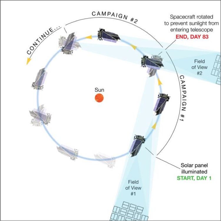
The K2 mission will observe sequential ecliptic campaigns with a duration of ∼83 days, where 75 days are dedicated to science.

The K2 mission will observe sequential ecliptic campaigns with a duration of ∼83 days, where 75 days are dedicated to science.

I’m a bit late to the game on this one, but I wanted to read Howell et al.’s (2014) paper describing the planned K2 mission, what is essentially the reincarnation of the Kepler mission.

Launched in 2009, the Kepler spacecraft was happily staring at about 150,000 target stars over about 4 years, looking for the shadows of planets as they passed between the Earth and their host star (called planetary transits). Groups using Kepler data have found thousands of planets outside our solar system, revolutionizing exoplanet studies. Unfortunately, two of the reaction wheels used to keep the spacecraft pointing stably at its target field failed by May 2013, ending the nominal science mission.

However, by carefully angling the telescope (see figure at left) and keeping it pointed along its orbital plane, NASA engineers realized they could use the photon pressure from Sun as a sort of third reaction wheel, allowing the astronomical revolution to continue — thus was born the K2 mission, which NASA selected for funding May this year.

The paper from Howell et al. (2014) describes the scientific and engineering capabilities of the K2 mission, which closely match those of the Kepler mission. So a lot of what Kepler could do, K2 can, too. In fact, since mission engineers have to turn the spacecraft every 80 days to satisfy the pointing requirements, K2 will look at lots of different fields on the sky, in contrast to Kepler, which only stared at the same field.

This variable pointing will enable a wider variety of scientific investigations, as discussed by Howell et al., including looking for more transiting planets, but also studies of other galaxies, supernovae, stellar clusters, and more. In fact, the astronomical community submitted more than 100 different ideas of things to do with K2. So the scientists and engineers at NASA have really done a spectacular job salvaging what otherwise would have been a disappointing loss.

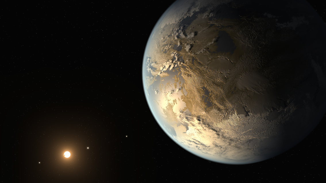
Artist’s conception of a habitable exoplanet in orbit around its red dwarf star. Credit: NASA Ames/SETI Institute/JPL-Caltech. From http://themeridianijournal.com/2014/04/big-discovery-first-earth-sized-exoplanet-habitable-zone-another-star/#more-5509.

Artist’s conception of a habitable exoplanet in orbit around its red dwarf star. Credit: NASA Ames/SETI Institute/JPL-Caltech. From http://themeridianijournal.com/2014/04/big-discovery-first-earth-sized-exoplanet-habitable-zone-another-star/#more-5509.

Interesting paper from Prof. Michael Jura at UCLA and colleagues, in which they look for the chemical signatures of plate tectonics in white dwarfs that are accreting planetary and asteroidal material. The paper presents a really neat idea, combining several big concepts.

First, there is strong evidence that several white dwarfs (the ghostly remnants of Sun-like stars) are accreting rocky materials. The atmospheres of white dwarfs are very simple, hot hydrogen and helium cooling to space over billions of years. Any other, heavier elements quickly settle out of the atmospheres (on timescales of millions of years), and so if you find such, heavier elements in the atmospheres (via spectroscopy), those elements were probably recently dumped into the atmosphere — a process called pollution.

Such pollution has been observed for many white dwarfs, and the pollution typically consists of rocky elements, silicon, magnesium, etc. Consequently, the polluting materials probably come from rocky asteroids, falling into the white dwarfs. Jura and colleagues point out that some of the pollution may arise from the crusts of extrasolar rocky planets orbiting the white dwarfs, in the form of debris from large impacts with the planetary surfaces.

Second, on the Earth, the constant subduction and eruption of crustal materials from plate tectonics has the effect of sieving out certain elements and leaving them in the crust, producing a crustal composition distinct from that of other planets and asteroids.

Jura and colleagues went looking for such a chemical signature in the rocky pollution of white dwarfs but unfortunately don’t find it. However, this initial study may provide a novel to search for the signs of plate tectonics in other planetary systems. That’s important because plate tectonics is thought to be a key requirement for making a planet suitable for life, but observing it astronomically is almost impossible (there’s no strong evidence any solar system planets other than Earth experienced/s plate tectonics). Jura and colleagues may have provided us a new way to peer into the geophysical histories of extrasolar planets.


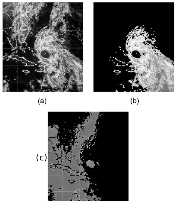
As part of my new push into data science, I read Shi & Malik’s paper on the perceptual grouping problem in which they develop a new algorithm for dividing an image up into coherent regions.

A portion of Figure 8 from Shi & Malik (2000).

A portion of Figure 8 from Shi & Malik (2000).

What does it mean to divide an image into coherent regions? Say, for example, you had a satellite image of a large storm system, such as the figure at left from Shi and Malik’s paper. Panel (a) shows the original image, while (b) and (c) show two portions of the image grouped together by Shi and Malik’s algorithm. The result makes intuitive sense (at least, to me): (b) is a large part of the storm, while (c) is the ground underneath.

Basically, Shi and Malik’s algorithm treats the entire image as a weighted graph, with portions of the image treated as nodes. Weights on the edges connecting the nodes are larger for portions that are closer to each other and for portions that are similar (where similarity may depend on the pixel brightnesses, textures, colors, etc.).

The algorithm decides which portions belong together as one segment using the weights for all the nodes connected in that segment. Shi and Malik developed a clever way to turn this process into an eigenvalue/vector problem, thereby dramatically facilitating the calculation. Their technique amounts to treating the pixels as individual masses connected by springs, with spring constants given by the edge weights, and then finding the normal modes of oscillation for the system: pixels that are strongly coupled are grouped together as one segment.

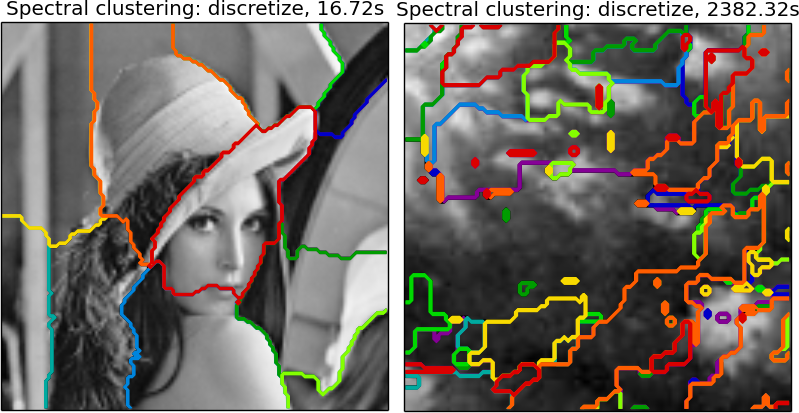
Conveniently, the algorithm is implemented in the scikit-learn python module. Using their example code, I was able to reproduce the segmentation of the Lena image easily (shown below), so I thought to try it on some VIMS observations of Titan. (Here’s the original Titan image. I took a small portion of it.)

Unfortunately, the result was not promising: the algorithm did NOT break up the image into the segments I expected. Instead, the segments seem pretty random. It also took about 40 minutes to work, even though the Titan image is smaller than the Lena image (100 x 100 pixels vs. 128 x 128).

(Left) Result from the spectral clustering example code on the scikit-learn page. (Right) My own attempt at segmenting a VIMS image of Titan.

(Left) Result from the spectral clustering example code on the scikit-learn page. (Right) My own attempt at segmenting a VIMS image of Titan.

Next things to try: it seems the algorithm needs me to tell it how many regions to use — I used the number given in the original example, 11. Maybe I should try a smaller number. There are also a few options as to how the graph weight are calculated in the original Shi and Malik algorithm (not sure if the scikit-learn module has that capability).

A mosaic from the Dawn mission of the asteroid Vesta.

A mosaic from the Dawn mission of the asteroid Vesta. From http://en.wikipedia.org/wiki/4_Vesta#mediaviewer/File:Vesta_full_mosaic.jpg.

Fascinating talk today from Roger Fu, a graduate student in MIT’s Earth, Atmospheric, and Planetary Sciences Dept, about magnetic fields in the solar system’s infancy.

Magnetic fields in the early solar system may have arisen from many sources, including the young Sun, the protoplanetary gas disk, and large planetary bodies like the asteroid Vesta (at left). The signatures of these magnetic fields were imprinted on meteorites present at this time, exactly the way molten rocks on the Earth can record the Earth’s magnetic field.  These ancient magnetic fields are called paleomagnetic fields.

By studying the paleomagnetic signatures imprinted on meteoritic materials, Fu and his colleagues are able to measure the strengths and even directions of magnetic fields in the early solar system. Understanding this early magnetism can teach us about the formation of planets, the evolution of the protoplanetary disk from which they formed, and even about how planetary magnetic fields themselves are generated.

Coma around Comet 17P/Holmes, 2007/11/02. From http://en.wikipedia.org/wiki/Coma_%28cometary%29#mediaviewer/File:17P-Holmes_Auvergne_2007_11_02.jpg.

Coma around Comet 17P/Holmes, 2007/11/02. From http://en.wikipedia.org/wiki/Coma_%28cometary%29#mediaviewer/File:17P-Holmes_Auvergne_2007_11_02.jpg.

Interesting talk today from Dr. Gorden Videen of the Army Research Lab. Dr Videen is an expert in the interaction of aerosols with light, particularly in their scattering and polarization properties.

Scattering of light by aerosols is something most people are familiar: if you’ve ever walked around your house shortly after sunrise, you have probably noticed dust motes drifting through your house. The motes seem to disappear later in the day. What’s happened is that, as the sun climbs into the sky, the angle at which sunlight strikes the Earth’s surface increases, and the light scattering properties of dust render it less visible. Dr. Videen uses the basic principles to glean knowledge about a variety of aerosol particles, from spores to volcanic eruptions.

Dr. Videen talked at length about his studies of cometary dust. For example, observations of comets like Comet Holmes have suggested that the sizes of particles released from the comet as its gas jets erupt can evolve over time, reflecting the interactions between the jets and particles. Thus, we can use the same physics that shows you how dusty your house is to study gaseous explosions on comets.

Predicted fatality counts. MFI indicates masculinity-femininity index (1 -> very masculine name, 11 -> very feminine name), and hurricanes with low MFI (vs. high MFI) are masculine-named (vs. feminine- named). Predicted counts of deaths were estimated separately for each value of MFI of hurricanes, holding minimum pressure at its mean (964.90 mb).

Predicted fatality counts. MFI indicates masculinity-femininity index (1 -> very masculine name, 11 -> very feminine name), and hurricanes with low MFI (vs. high MFI) are masculine-named (vs. feminine- named). Predicted counts of deaths were estimated separately for each value of MFI of hurricanes, holding minimum pressure at its mean (964.90 mb).

We discussed a very interesting paper today in Journal Club, Jung et al.’s (2014) study of correlations between the perceived masculinity-femininity of a hurricane’s name and its death toll. As reflected in the figure at left from the paper, the higher the masculine-feminine index for a hurricane (MFI, 1 -> very masculine name, 11 -> very feminine name), the larger the predicted fatality count. As a specific example, Jung et al. estimated that Hurricane Eloise (with a decidedly female MFI = 8.944) killed three times as many people as Hurricane Charley (MFI = 2.889).

Jung et al. also polled participants and found they consistently rated female storms as less likely to be severe and indicated they were less likely to evacuate in the wake of female storms, perhaps due to implicit gender biases. Ostensibly, their results suggest a lot of lives could be saved by simply not using female names for hurricanes.

But there are a lot of questions that were not addressed by the study, and others who have looked at the data have pointed out important unresolved issues.

A blog entry at Prooffreader.com pointed out that the authors should only have considered hurricanes after 1979 since there were no male hurricane before then. The blogger showed that, comparing total hurricane deaths since both male and female names have been used (1979), male hurricanes killed more people (413 total) until just two years ago, when Hurricane Sandy brought the total for females to 459. And this result used the authors’ own data.cum_alldeaths The plot at right is a recreation of the Prooffreader.com plot.

I spent several hours yesterday, poring over the paper and have to admit that I did not understand the statistical methods employed. The authors don’t give a lot of details, and the key references for the techniques seem to be two textbooks to which I don’t have access.

The paper talks about using a model to estimate the number of deaths for a storm of a given severity, but to the extent that I can compare their predicted death tolls to actual, the model seems pretty discrepant with the data. For example, their model estimates that Hurricane Eloise killed 41.45, but the actual number killed was 21. They also estimated Hurricane Charley killed 14.87, whereas Hurricane Charley from 1986 killed 5 and the one from 2004 killed 10 (they don’t say which Charley they meant).

So Jung et al. present a very interesting idea, but it’s not at all clear that their results hold up. I’m sure this paper will prompt a spat of sociological studies into hurricane statistics, though, which will probably lead to additional disaster preparedness and save lives.


M87_jet

Hubble Space Telescope image of a 5000-light-year-long (1.5-kiloparsec-long) jet being ejected from the active nucleus of the active galaxy M87. From http://en.wikipedia.org/wiki/Active_galactic_nucleus.

Great talk today from Dr. Eileen Meyer of Space Telescope Science Institute (STScI) about gaseous jets launched from active galactic nuclei AGN.

These cosmic monsters emit a lot of matter and energy, sometimes in the form of jets (see picture at left) that can outshine the rest of the host galaxy. The jets can be observed to span vast distances, thousands of light years, larger than the host galaxies themselves, and mounting evidence suggests that the jets are powered by supermassive blackholes, living deep within the galaxy.

Meyer studies the evolution of these jets, and by following the motions of individual clouds of gas, she can tease out their velocity vectors, critical for understanding the amount of energy and momentum carried by the jets. In some cases, she’s found that the jets can brighten or fade over just a few years, some of the few astronomical objects that can be observed to change appreciably on human timescales.

Understanding the detailed properties of these jets is critical because they are so powerful they can shape the growth of galaxies and even in the evolution of the Universe itself over the largest spatial and temporal scales.

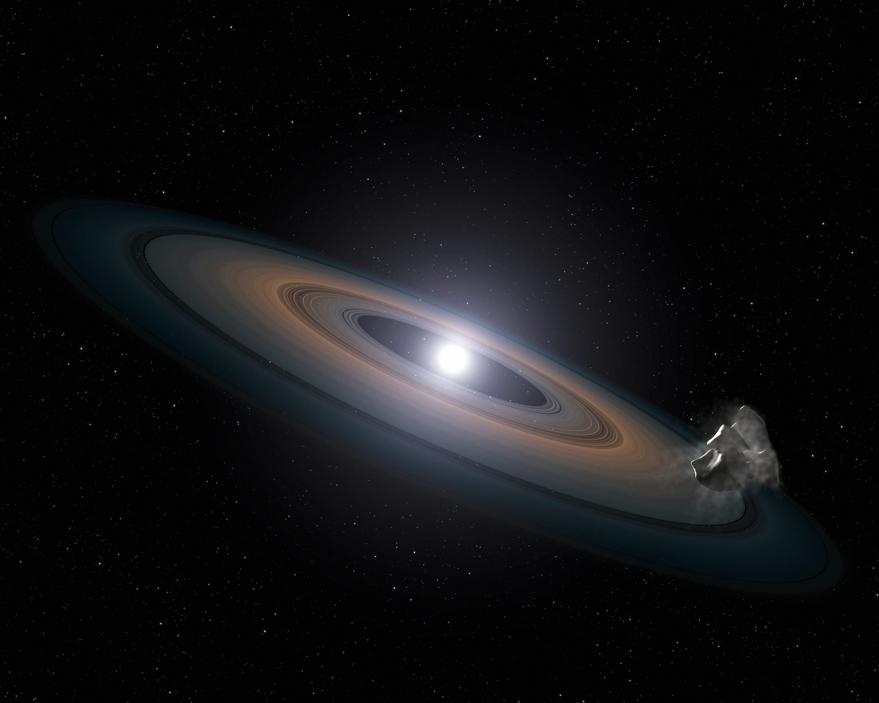
This illustration is an artist's impression of the thin, rocky debris disc  discovered around the two Hyades white dwarfs. Rocky asteroids are  thought to have been perturbed by planets within the system and diverted  inwards towards the star, where they broke up, circled into a debris  ring, and were then dragged onto the star itself. From http://en.wikipedia.org/wiki/File:Artist%E2%80%99s_impression_of_debris_around_a_white_dwarf_star.jpg.

This illustration is an artist’s impression of the thin, rocky debris disc discovered around the two Hyades white dwarfs. From http://en.wikipedia.org/wiki/File:Artist%E2%80%99s_impression_of_debris_around_a_white_dwarf_star.jpg.

Fun talk today from Dr. John Debes from the Space Telescope Science Institute (STScI) about white dwarfs eating planetesimals.

White dwarfs are the ghostly embers of former stars — they originate when a star (that is small enough not to become a black hole instead) dies and leaves behind a dense core of carbon and oxygen, enshrouded in a thin hydrogen atmosphere. That white dwarf core then slowly cools and darkens over billions of years, basically doing nothing else.

However, many white dwarfs show telltale signs in their atmospheric spectra of rocky materials. Debes, along with others, has suggested that material arises from asteroids that are perturbed by distant planets around the white dwarf. Those orbits take the asteroids so close to the white dwarf host that they are ripped apart by the star’s gravity, producing a cloud of dust and gas that then accretes onto the star.

Astronomers can very accurately measure the composition of that dust, which can actually tell us something about the compositions of asteroids in distant planetary systems. So astronomers can learn about what makes up the planets in distant systems by studying the remains in these planetary graveyards.

Possible processes and chemical reactions in the martian atmosphere. From Villanueva et al. (2013 -- http://www.sciencedirect.com/science/article/pii/S0019103512004599).

Possible processes and chemical reactions in the martian atmosphere. From Villanueva et al. (2013 — http://www.sciencedirect.com/science/article/pii/S0019103512004599).

Great talk today from Dr. Gerónimo Villanueva from NASA Goddard Space Flight Center on organics on Mars.

Villanueva was on the team that reported discovery of methane in the atmosphere of Mars. This discovery is important because methane is thought not to stick around too long on Mars (< 300 years), and so something has to actively produce it for methane to be there now, such as microbial life.

Detecting methane on Mars is difficult from telescopes on the ground on Earth because the Earth’s atmosphere also has a lot of methane in it. In order to see the Martian methane, Villanueva has to do a lot of observing and modeling to rescue the tiny spectral signal of Martian methane from underneaththe whopping terrestrial signal.

According to Villanueva, current observations suggest that, if methane is released into the Martian atmosphere, it is released rarely and not seasonally. In his most recent work, Villanueva did not detect any methane, possibly indicating that methane has an even shorter lifetime in the Martian atmosphere than previously thought. And so work continues to understand this puzzling but tantalizing discovery.