AAS 225 — Day -2

python.sh-600x600The new year finds me in Seattle two days before the AAS 225 meeting officially begins to attend the Software Carpentry workshop. This workshop is put on by a volunteer organization that teaches scientists how to write and maintain robust code.

On the first day, we covered some shell scripting, basic python, and the ipython notebook. Just the first few lessons are already hugely useful for me, and the teachers are doing a great job explaining things clearly. They are also using a variety of tools to record and document the workshop. I’ve pasted links to those records below.

Very much looking forward to Day 2.

Useful links and particularly useful notes:

Total amount of water lost for a 1 Earth-mass planet.

Total amount of water lost for a 1 Earth-mass planet.

In journal club on Friday, we discussed a fascinating paper that presented some problematic results for detecting life on other planets. Luger and Barnes (2014) looked at what could happen to the water on Earth-like planets orbiting many different kinds of stars.

Like the Sun, all stars produce x-rays and ultraviolet light (UV), but not all stars produce the same amount. In fact, stars much less massive than the Sun produce a lot more.

That’s a problem for life on planets orbiting these stars because x-rays and UV (collectively called XUV) can photodissociate (or break-up) water molecules in the atmosphere. Once the water is broken into hydrogen and oxygen atoms, the hydrogen can escape to space so the water is permanently lost, leaving behind the oxygen.

And this isn’t just a hypothetical scenario — Venus probably had oceans, like the Earth, and lost them this way. Of course, water is necessary for life as we know it, so a planet that loses its water can’t host life.

Luger and Barnes modeled this process and found that a lot of planets that might otherwise be suitable for life could actually lose a lot of water. The figure at left shows how much water could be lost for planets in the habitable zones of stars from about 0.1 to 0.9 solar masses (M⊙). The dark red region shows that most of the planets would actually lose at least 1 oceans-worth of water.

So not only would these planets be bone-dry, they could have a lot of oxygen in their atmospheres. On the Earth, oxygen is produced by photosynthetic planets and algae, and so its presence in a planet’s atmosphere is usually thought of as a smoking gun for life. If Luger and Barnes are right, their results may spell trouble for the search for life elsewhere in the universe.

The Chariklo ring system. The dotted lines are the trajectories of the star relative to Chariklo in the plane of the sky, as observed from eight sites, the arrow indicating the direction of motion.

The Chariklo ring system. The dotted lines are the trajectories of the star relative to Chariklo in the plane of the sky, as observed from eight sites, the arrow indicating the direction of motion.

We discussed a marvelous paper in journal club on Friday — Ribas-Braga et al.’s discovery of a ring system around the Centaur Chariklo.

A small icy body in the outer reaches of our solar system, Chariklo was expected to occult a star last year as seen from the Earth. The shape and duration of this stellar dimming can give astronomers very tight constraints on the size of a body (the same basic technique is used in exoplanet astronomy to estimate planet sizes).

Instead of one very deep dimming due to Chariklo itself, the observers were surprised to find two pairs of small dips just before and after Chariklo’s dip. Follow-up observations at other sites confirmed what these initial observations suggested: Chariklo has two, thin rings! This result makes Chariklo the only body in the solar system, other than the giant planets, known to have a ring system.

A ring system around such a small body is very surprising, and it’s not at all clear how it was made — possibly tidal disruption of an even smaller icy body or collisions among small satellites; both scenarios may have contributed to Saturn’s rings.

And like Saturn’s ring system, Chariklo’s rings may have shepherding satellites, gently tugging and pushing the ring particles to keep them tightly confined around Chariklo. Otherwise, such a ring system should spread out and diffuse in only a few million years.

One of the most exciting aspects of this paper for me was the fact that the occultation observations were mostly made by small telescopes. Boise State has its own 0.4-m telescope at the Challis Observatory. And so I’m hopeful we may be able to contribute to future occultation campaigns such as this one.


The broad-band transmission spectral data of WASP-31 b, along with three atmospheric models. From Sing et al. (2014 -- http://arxiv.org/abs/1410.7611).

The broad-band transmission spectral data of WASP-31 b, along with three atmospheric models. From Sing et al. (2014 — http://arxiv.org/abs/1410.7611).

We discussed an impressive paper today in journal club, Sing et al.’s (2014) study of the transiting, hot Jupiter WASP-31 b.WASP-31 b weighs about half as much as Jupiter but has a radius more than 50% larger, giving it a very low density for a Jupiter-like planet.

Using the Hubble Space Telescope, Sing and colleagues observed several, spectrally-resolved transits of WASP-31 b (i.e., in several different colors), resulting in several of the black data points in the figure at left.

The colors of the planet’s transit tells us a lot about the composition and nature of WASP-31 b’s atmosphere. For example, the blue and green curves in the figure at left include spectral features from water, but the black data points don’t show the same features.

However, the data points DO show a clear detection of potassium (K) in the planet’s atmosphere (as indicated in the figure). Potassium, while interesting, is not completely unexpected in WASP-31 b’s atmosphere since it is very hot, > 1,500 K.

But the fact that only the very highest point in the potassium spectral feature is seen and not the broad wings on either side probably indicates the planet has a thick cloud deck. Since the peak of the potassium feature results from gas high in the planet’s atmosphere and the wings from lower in the atmosphere, Sing and colleagues can estimate the pressure level of the cloud deck, about 10 mbar.

For comparison, clouds on the Earth typically form at about 500 mbar. In the Earth’s atmosphere, 10 mbar is about the level where meteors burn up, so WASP-31 b’s clouds are VERY high in its atmosphere.

The full set of rings, imaged as Saturn eclipsed the Sun from the vantage of the Cassini spacecraft. Earth is visible as a "pale blue dot" at about the 4 o'clock position. From http://en.wikipedia.org/wiki/Rings_of_Saturn.

The full set of rings, imaged as Saturn eclipsed the Sun from the vantage of the Cassini spacecraft. Earth is visible as a “pale blue dot” at about the 4 o’clock position. From http://en.wikipedia.org/wiki/Rings_of_Saturn.

For our inaugural journal club at BSU physics, we discussed a very interesting paper led by Prof. Matt Hedman, now at University of Idaho Physics.

Hedman and Nicholson studied subtle density perturbations in Saturn’s ring system. If you look at images of the rings, you’ll see lots of patterns, many of which are caused by gravitational interactions with Saturn’s many satellites — the inner edge of the Cassini division, for example, is sculpted by gravitational tugs from Mimas.

However, the ring patterns studied by Hedman and Nicholson seem to result from gravitational perturbations with periods much shorter than the orbital periods of any Saturnian satellite, meaning the satellites aren’t the cause.

The periods actually correspond to those expected for oscillations within Saturn itself. Just like stars exhibit oscillations, Saturn oscillates, producing periodic variations in its gravitational field. And, as for stars, the periods of these oscillations depend on its interior. So by studying these subtle ring patterns, Hedman can tease out information about Saturn’s internal structure.

Hedman has coined the term “Kronoseismology” for this new approach to studying Saturn’s interior, analogous to “asteroseismology” for stars and “seismology” for the Earth. And just like those fields, Kronoseismology promises to lead to profound new insights about the second biggest planet in our solar system.

The density of Bose-Einstein condensates, exhibiting interference of their quantum mechanical wave functions. From https://sites.google.com/site/bigelowcatgroup/bec.

The density of Bose-Einstein condensates, exhibiting interference of their quantum mechanical wave functions. From https://sites.google.com/site/bigelowcatgroup/bec.

BSU’s Materials Science and Engineering Dept had a guest today from the University of Rochester, Prof. Nick Bigelow. Prof. Bigelow spoke this afternoon in the physics department about his experiments producing Bose-Einstein condensates in his optics lab. He did a great job of explaining their subtle physics at a level that our undergrads and even our lowly astronomers could understand.

In his lab, he uses lasers to cool small pockets of low-density rubidium gas to a Bose-Einstein condensation state and then spins up a torus of the gas with variously polarized laser beams. The quantum mechanical wave function describing the gas torus must then have an integer number of oscillations over its circumference.

By putting the spinning torus of gas into contact with other Bose-Einstein condensates with known wave functions (either spinning or not), Bigelow’s group can demonstrate the effects of interference between the quantum mechanical wave functions for the two condensates. The figure at top left shows the clouds of gas that form, exhibiting graceful density enhancements (warmer colors) that result from interference of the wavefunctions.

As lucid and compelling as Bigelow’s talk was, it highlighted again for me how strange and counter-intuitive quantum mechanical systems are. It reminded me of Richard Feynman‘s famous quote, “If you think you understand quantum mechanics, you don’t understand quantum mechanics” (which, I just learned, is not a Feynman quote at all, but a paraphrase of a Bohr quote).

I really enjoyed a talk from Dr. Josh Bandfield yesterday in the Geosciences Department about unusual geomorphological features on the surface of the Moon.

Bandfield works with the Diviner instrument onboard the Lunar Reconnaissance Orbiter. Diviner is a very sensitive camera that measures infrared radiation from the Moon’s surface over a wide range of wavelengths. Using these data, Bandfield and others can learn a surprising amount about the Moon’s surface and geological history.

Rock concentration values near Rima Bode (356.1°E, 12.9°N) superposed on a high-res LROC image. The white box denotes the area shown in the bottom image. (bottom) A portion of LROC image. Each square in the image covers a separate Diviner bin with the derived rock concentration value listed.

Rock concentration values near Rima Bode (356.1°E, 12.9°N) superposed on a high-res LROC image. The white box denotes the area shown in the bottom image. (bottom) A portion of LROC image. Each square in the image covers a separate Diviner bin with the derived rock concentration value listed.

For example, the rates at which different surface types cool once the Sun sets depend on the surfaces’ thermal conductivity. In general, lunar regolith or soil heats up and cools down much more quickly than bare rock. And so, if Diviner measures a surface’s temperature at a known time of lunar day, Bandfield can determine how rocky the surface is. The figure at left from Bandfield et al. (2011) compares the inferred rockiness of one surface to high-resolution images, which confirm the rockiness map from Diviner data.

Bandfield also discussed how rockiness maps can be used to determine the relative ages of lunar craters. Since the Moon is constantly bombarded by impactors, lunar rocks are continually broken down into finer and finer pieces, finally turning into powdery regolith. By mapping the rockiness of different craters, Bandfield and colleagues found the youngest craters are also the most rocky.

A theme that Bandfield highlighted several times: even though humans have studied the Moon for millenia, it still has fascinating things to reveal.

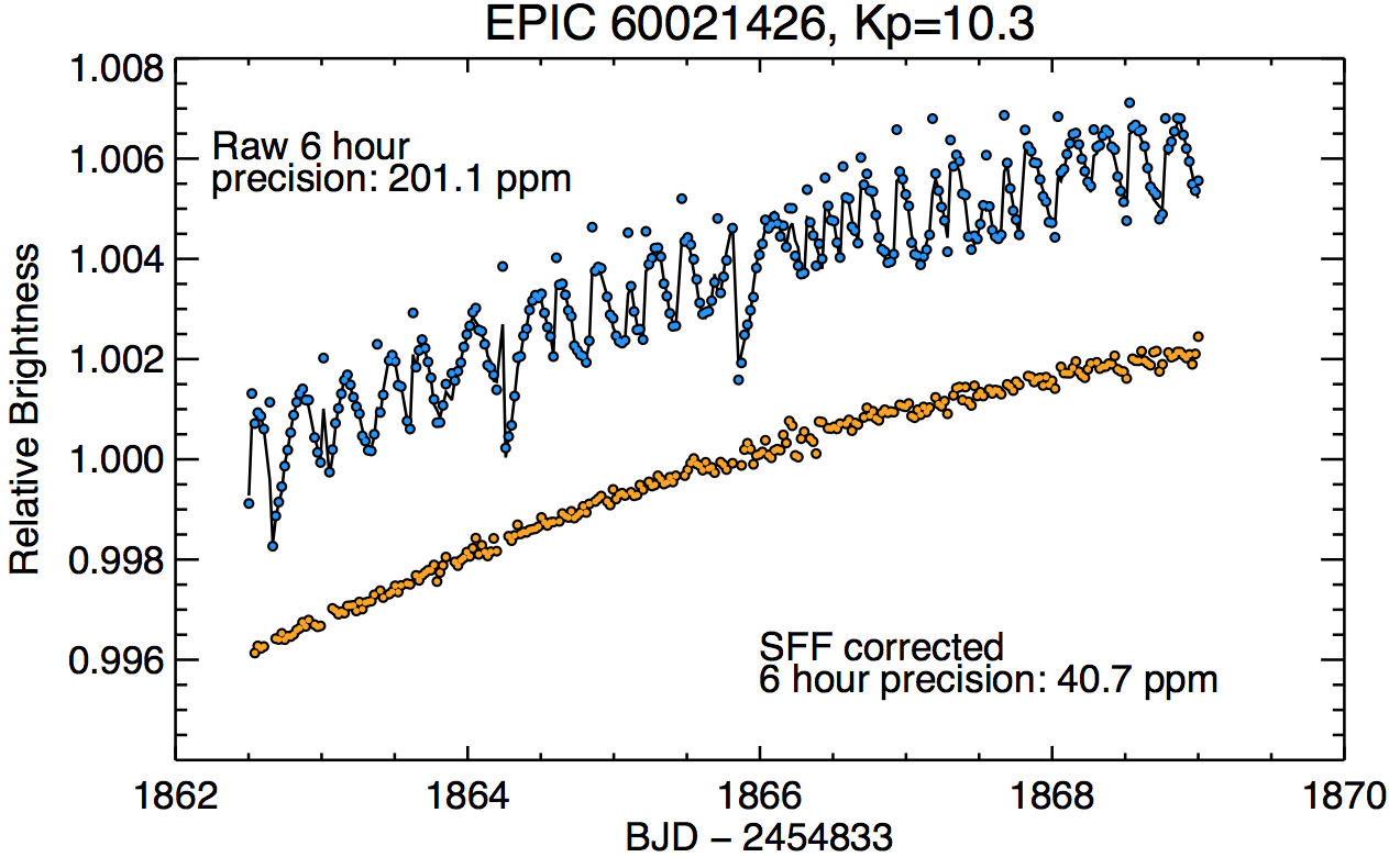
Comparison between raw K2 and corrected photometry. Figure 5 for Vanderburg & Johnson (2014).

Comparison between raw K2 and corrected photometry. Figure 5 for Vanderburg & Johnson (2014).

Read a neat paper from Andrew Vanderburg of John Johnson’s Exoplanets group at Harvard about working with data from the upcoming K2 mission.

Having suffered failures of two of its reaction wheels, required to accurately point the telescope, the Kepler mission has ended its nominal science investigation. However, clever engineering will allow the spacecraft to keep operating and doing exciting astronomy as the K2 mission.

Among other goals, the K2 mission will continue to look for transiting exoplanets, which involves looking for the shadows of planets as the occult their host stars. However, small attitude tweaks needed to keep the K2 spacecraft accurately pointed result in fairly large artificial variations in the measured brightnesses of target stars. Removing the effects of these tweaks from K2’s data can be quite challenging, but Vanderburg & Johnson’s recent paper describes one technique for doing that.

By carefully tracking the centers of target stars as they drift across the K2 CCD camera, their technique allows them to remove quite large and complex artificial variability and to recover the actual brightness variations of target stars.

From the paper, the figure at left shows how well they do: the blue dots at the top show the raw measurements, with the artificial variations from attitude tweaks apparent as discontinuous jumps. By carefully modeling the exact position of the target star and removing the effects of its motion across the CCD, the technique produces a much more accurate measurement of the actual brightness variations of the target star, orange dots at bottom.

Applying these techniques to many target stars monitored during one of the K2 engineering tests, Vanderburg & Johnson showed they can produce data nearly as precise as the original Kepler mission — almost as good as sending an astronaut repair team to fix the Kepler spacecraft, but all it took was some sophisticated numerical modeling and a laptop.

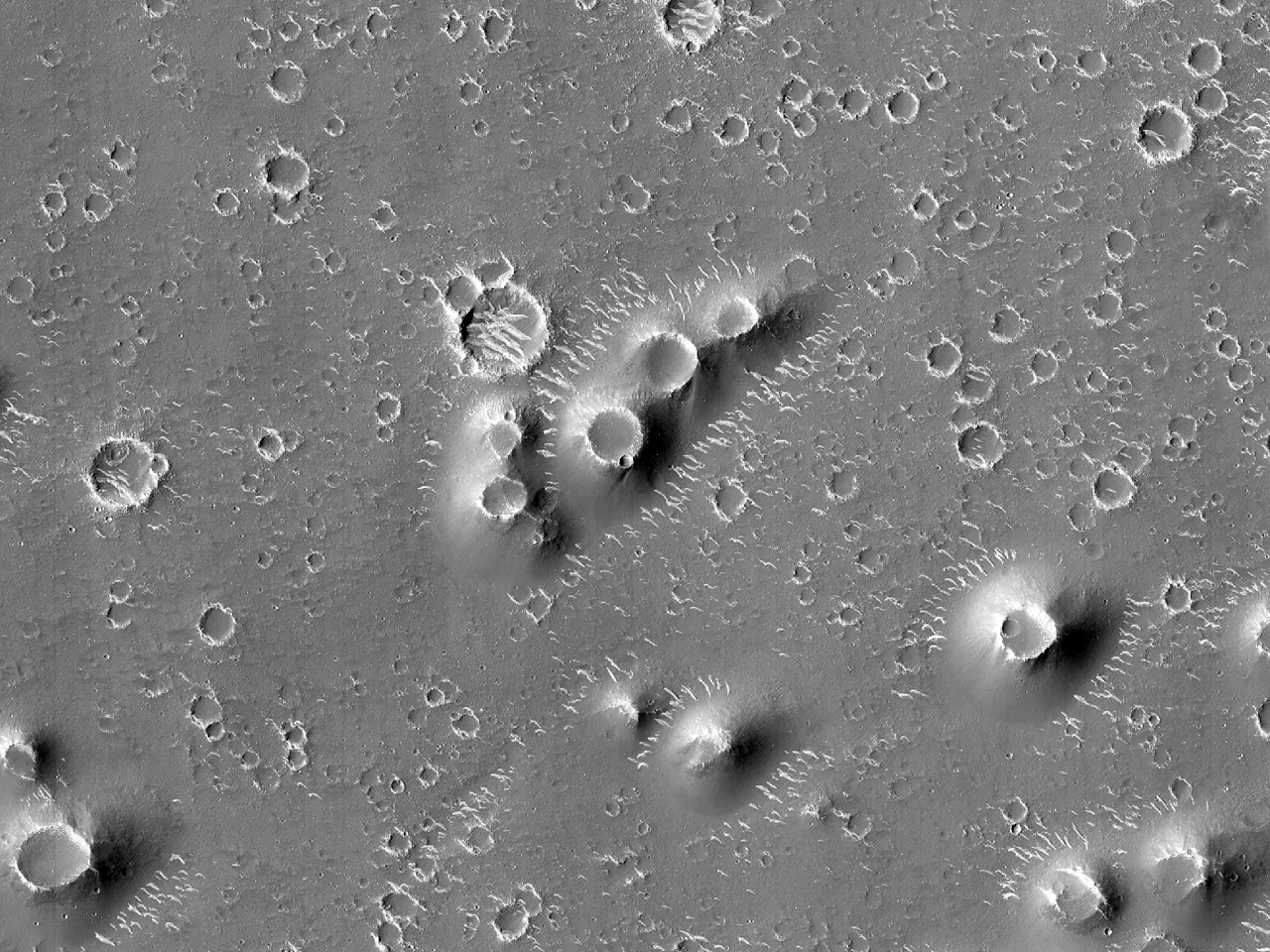
A field of pitted cones in Utopia Planitia on Mars, as observed by the HiRISE instrument onboard the Mars Reconnaissance Orbiter. Taken from http://beautifulmars.tumblr.com/post/82817530060/field-of-cones-in-utopia-planitia.

A field of pitted cones in Utopia Planitia on Mars, as observed by the HiRISE instrument onboard the Mars Reconnaissance Orbiter. Taken from http://beautifulmars.tumblr.com/post/82817530060/field-of-cones-in-utopia-planitia.

A visit from a planetary sciences colleague this weekend got me excited again about automated feature identification for remote-sensing imagery. This colleague and I talked about her work on Martian pitted cones (examples shown at left). These small hills form when a basalt flow passes over volatile (i.e., water) deposit, heating it and producing a steam explosion that uplifts the flow into a cone shape with a crater at the apex.

As for the vast majority of geomorphological studies, pitted cones on Mars are identified by groups of dedicated researchers, sifting by hand through hundreds or thousands of high-resolution images. If, instead, identification could be automated, it would help realize dramatic savings in person-hours and probably significantly increase the number of known features. It could also mitigate potential observational biases introduced by human image processing.

As an experiment, I applied algorithms from the scikit-image python package to find pitted cones in the example image shown at left. Fortunately, the documentation already provides a good example of circular feature detection.

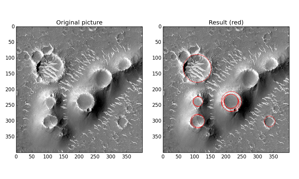
So modifying the example code, I applied it to a small portion of the example image, and the figure below shows the results. Here I’m just showing the top ten most strongly detected circular features.

Unfortunately, the algorithm is not perfect — some of the obvious cones were not picked out, and others were highlighted more than once. But overall, not terrible, considering it took me about an hour and a half to implement (which included upgrading to Python 3 via the Anaconda package because scikit-image wouldn’t work with the Enthought Python version 2.7 — this upgrade will probably adversely affect my ability to use astroml, by the way).

Possible ways to improve things:

  1. The example code only returns the top two most strongly detected features for each circle radius it tries; this restriction would be simple to remove.
  2. The fact that the pitted cones are cone-shaped means you could require that any putative crater be framed by an appropriately shaped shadow. Regardless of the cone’s actual height (probably unknown anyway), the shadow on the cone should darken as the solar incident angle approaches 180 degrees, modulo any nearby morphological features (as evident in the figure below).
My attempt to automatically identify pitted cones using scikit-image.

My attempt to automatically identify pitted cones using scikit-image.

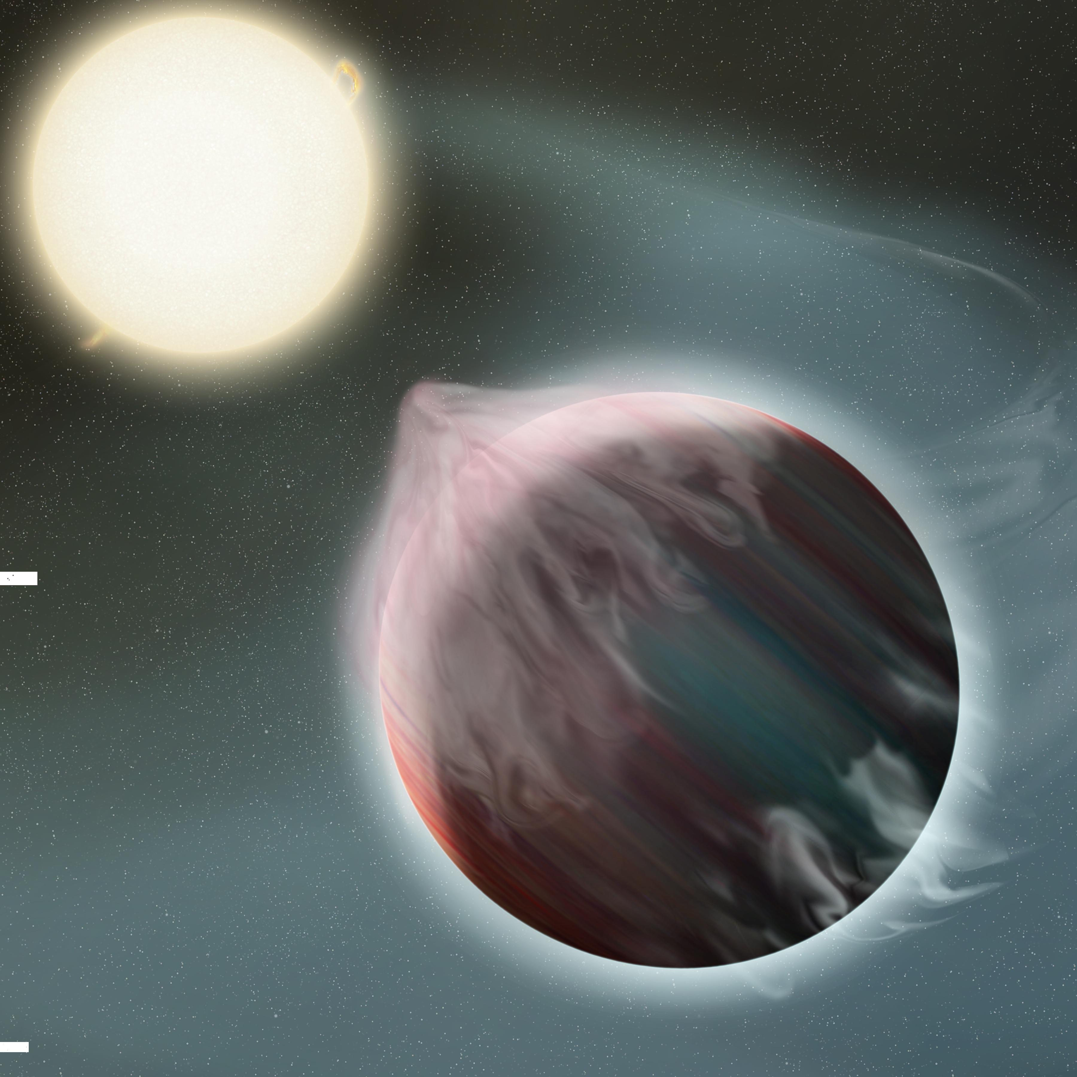
Artist's conception of tidal disruption of a gas giant planet.

Artist’s conception of tidal disruption of a gas giant planet.

Neat paper today from Francesca Valsecchi and colleagues at Northwestern University’s Center for Interdisciplinary Exploration and Research in Astrophysics. They looked at the final fates of gas giant planets that wander too close to their host stars, sometime called “hot Jupiters”.

This unexpected but apparently fairly common class of planet consists of massive planets made mostly of hydrogen and helium, like Jupiter, but, unlike Jupiter, these planets orbit tens or even hundreds of times closer to their host stars than the Earth orbits the Sun. Consequently, many of these hot Jupiters are fated to spiral closer and closer to their stars, eventually getting so close that their host stars’ gravity rips them apart, drawing their atmospheres into thin accretion disk around the star. This process is called “Roche lobe overflow” (RLO).

Once the progenitor hot Jupiter has lost its atmosphere, what’s left behind is probably the rocky/icy core at its center, and following up studies by other groups, Valsecchi and colleagues point out that RLO of hot Jupiters may help explain the puzzling presence of small rocky planets also found orbiting very close to their host stars. These little bodies may indeed be the skeletal remnants of unspeakable astrophysical violence.