exoplanets

All posts tagged exoplanets

At journal club, we discussed the discovery of two new hot Jupiters using data from ESA‘s CoRoT mission, with the names CoRoT-28 b and -29 b. Both systems seem a little off.

The host star CoRoT-28 has an inflated radius, suggesting it is ancient and on its way off the main sequence. But it has a lot more lithium than we’d expect for an old star, and its rotation rate is similar to the Sun’s, much faster than we would expect.

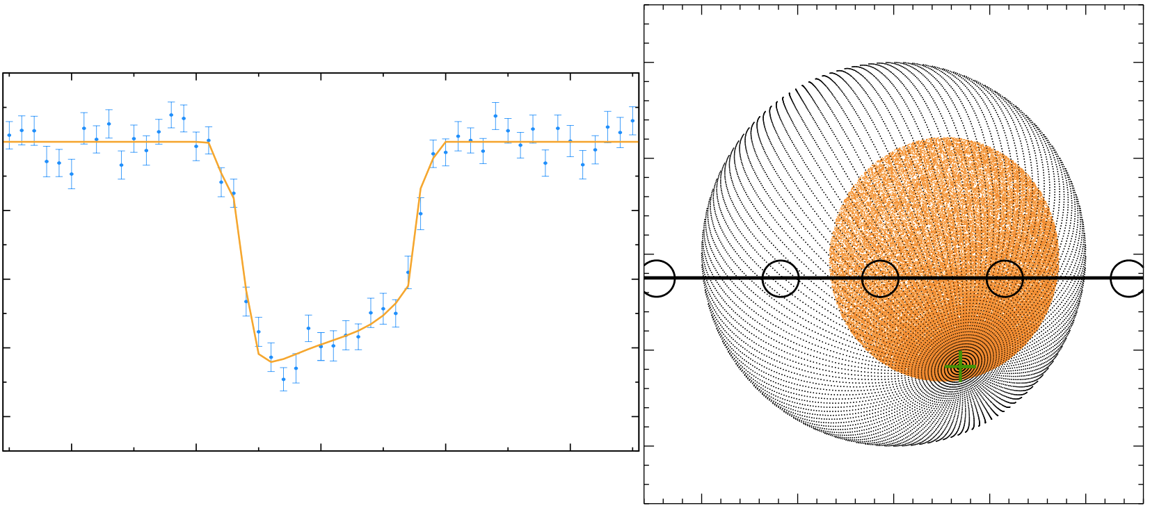
Equally puzzling is the transit light curve for CoRoT-29 b (shown below at left). Most transit curves are u-shaped, but CoRoT-29 b’s is strangely asymmetric. The asymmetry resembles what has been seen for a planet transiting a rapidly rotating star — rapid rotation reduces the gravity at the stellar equator, resulting in a cooler, darker region. Barnes et al. (2013) looked at the transit light curves for such a Kepler system and actually used the light curve to study the planet’s orbital inclination.

(left) CoRoT-29 b transit light curve. (right) Planet transiting star spot.

(left) CoRoT-29 b transit light curve. (right) Planet transiting star spot.

But CoRoT-29 doesn’t appear to be a rapid rotator. So instead Cabrera et al. suggest that perhaps the star has a large, nearly stationary star spot and that the planet transits the spot over and over again. However, this scenario would require a nearly stationary spot with a very long lifetime (~90 days), neither of which is expected.

So a few more astrophysical conundra to add to the growing list of puzzling exoplanet discoveries.

Journal club attendees included Jennifer Briggs, Emily Jensen, and Hari Gopalakrishnan.

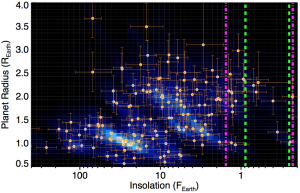
The radii of planets found in the Kepler dataset by Dressing & Charbonneau (2015) as a function of the amount of star light (insolation) they receive. The pink and green lines show ranges of insolation we think might allow the planets to be habitable.

The radii of planets found in the Kepler dataset by Dressing & Charbonneau (2015) as a function of the amount of star light (insolation) they receive. The pink and green lines show ranges of insolation we think might allow the planets to be habitable.

In journal club today, we discussed a recent study by Dressing & Charbonneau (2015) that used the Kepler dataset to search for possibly habitable planets around small (M-dwarf) stars.

Dressing and Charbonneau applied a sophisticated and comprehensive search scheme to look for habitable planets and estimate how effective their search was in finding such planets. Based on their analysis, they estimated that about 1 in 4 M-dwarf stars have planets about the size of Earth in their habitable zones and that the nearest such planet is about 8.5 light years away.

This is far enough that we’d probably still need a generation ship to reach it but a lot closer than one case, 20 light years to the nearest habitable planet, considered by Hein et al. (2012) in their analysis of interstellar colonization. This reduction in travel time could reduce the minimum population required to make the trip from maybe 7,000 to 4,000 people.

Of course, the habitable planet sought in such a trip would orbit a much cooler, redder star than the Sun, so the colonists should be prepared to plant very different crops than we have on Earth.

Attendees of today’s journal club included Simon Pintar, Nathan Grigsby, Jacob Sabin, Tyler Wade, Liz Kandziolka, Jennifer Briggs, and Emily Jensen.

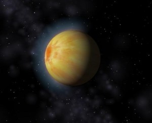
Artistic rendering of 51 Peg b, from http://en.wikipedia.org/wiki/51_Pegasi_b.

Artistic rendering of 51 Peg b, from http://en.wikipedia.org/wiki/51_Pegasi_b.

For the majority of exoplanets, astronomers study the planets via indirect means, by looking for their gravitational tugs on their host stars or the shadows they cast when occult their stars. Consequently, the things astronomers learn about exoplanets often involve systematic uncertainties, usually related to uncertainties about our knowledge of the stellar properties.

For example, by measuring a planet’s gravitational tugs on its star, astronomers can estimate the planet’s mass but only if they also know the star’s mass. It’s a little like watching two dancers spinning hand-in-hand, with one in black and the other in white,  and then trying to estimate the weight of the dancer in black based on how the dancer in white spins.

But in last week’s journal club, we discussed a recent study from Martins and colleagues that may have thrown white clothes on one of the most famous exoplanets, 51 Pegasi b, and revealed its dance moves.

51 Peg was the first exoplanet discovered around a Sun-like star. It’s a gas giant, like Jupiter, but unlike Jupiter, it orbits its host star every four days and is almost 100 times closer to its host star than Jupiter is to our Sun.

Martins and colleagues conducted ground-based spectroscopic observations of the 51 Peg system as the planet revolved about its host star. In principle, this orbital motion causes the spectral features imprinted on light reflected from the planet’s atmosphere to be Doppler-shifted.

Detecting the light reflected from a planet and resolving it spectrally is a bit like trying to discern the color of a football fan’s t-shirt against the glare of stadium lights, only much harder.

However, Martins and colleagues found tentative indications of light reflected from 51 Peg b’s atmosphere. By modeling the Doppler-shifting of the subtle spectral signals, they were able to estimate the planet’s mass (0.46 times Jupiter’s) and its radius (almost twice Jupiter’s, if it’s about twice as reflective as Jupiter).

Journal club attendees included Jennifer Briggs, Nathan Grigsby, Emily Jensen, and Liz Kandziolka.

At journal club today, we talked about a study from Heller and Pudritz that looks at the formation of moons around gas giant planets in extrasolar systems.

Heller and Pudritz modeled the conditions in circumplanetary disks around Jupiter-like planets to find where temperatures are right for icy moons like Jupiter’s to form. Like Goldilocks, moon formation requires conditions that are juuust right: the planet can’t be too close to its star or too small.

But given the right conditions, moons will happily accrete around a gas giant and the most massive circumplanetary disks around super-Jovian planets can form moons the size of Mars.

Heller and Pudritz point out that this means if we find an icy moon around one of the many gas giant exoplanets orbiting at about 1 AU from their host stars, we can infer the planet didn’t form there. Instead, it must have formed farther out and migrated in.

And at 1 AU around a Sun- like star, the discovery of such an exomoon would naturally make it a high priority target for habitability studies.

Attendees at today’s journal club included Nathan Grigsby, Jared Hand, Catherine Hartman, Emily Jensen, Liz Kandziolka, and Jacob Sabin.

Had fun playing with the telescope again last night on BSU’s campus.

This time, we observed 55 Cnc, one of very few naked-eye stars that hosts transiting exoplanets. 55 Cnc’s planetary system comprises five fairly large planets, including one twice the size and eight times the mass of Earth in an orbit that roasts its surface at a temperature of 2,360 K — hot enough to vaporize iron.

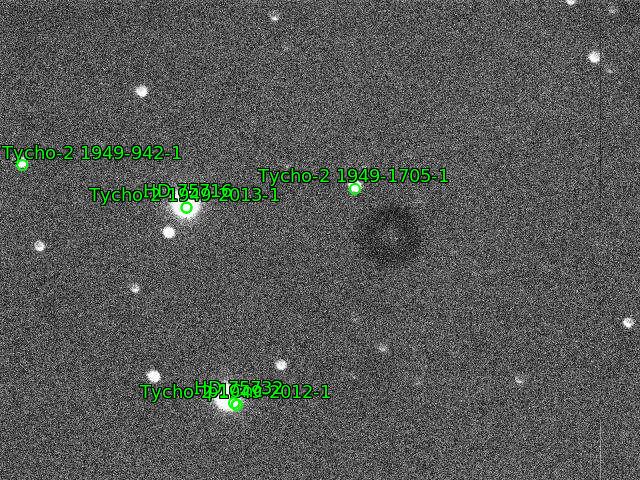
Below is our image of the sky, annotated by the astrometry.net service (try to ignore the dark doughnut that is probably a dust mote on the telescope). 55 Cnc is the bright star at the bottom and is also called HD 75732.

55 Cnc observed by BSU's campus.

55 Cnc observed by BSU’s campus.

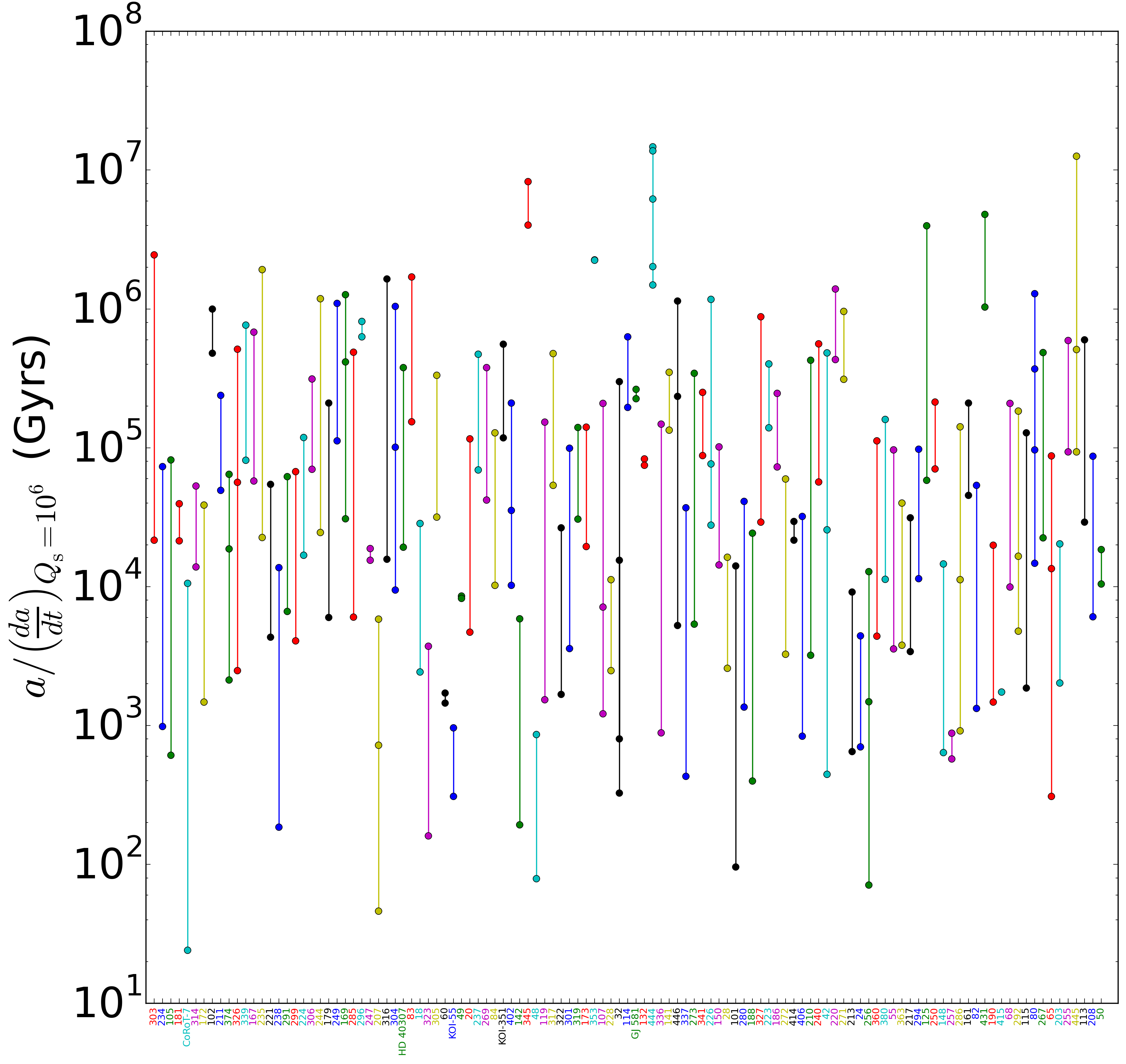
A preliminary investigation showed a project a colleague and I were considering probably isn’t worth doing. But for that investigation, I took a few hours to make a rather complicated plot using pylab, so I thought I’d share how I did that.

First, here’s the plot:

Tidal decay timescales for members of multi-planet systems.

Tidal decay timescales for members of multi-planet systems.

The plot shows the timescales for tidal decay of members of multi-planet systems. Unfortunately, the x-axis labels aren’t legible unless you zoom in, but if you do, you can see the font colors match up with the corresponding line colors.

Below is the ipython notebook I used to generate the plot. The excel spreadsheet with the data is here.

#Show the plot inline
%matplotlib inline

#load in the required modules
import pandas as pd
import pylab as pl
import itertools as it
import numpy as np

# using the ExcelFile class
xls = pd.ExcelFile('exoplanet-archive_2015Mar25.xlsx')
data = xls.parse('obj of interest', index_col=1)
data = data[pd.notnull(data['a/(da/dt)Qs=1e6 (Gyrs)'])]

#Make a nice, big figure
fig = pl.figure(figsize=(15,15))
ax = fig.add_subplot(1, 1, 1)

#Make a list, indexing the dataframe labels
indices = range(len(set(data.index)))

#Make a list with the indices as the entries
labels = list(set(data.index))
#For concision, drop "Kepler" wherever it's found
labels = [w.replace('Kepler-', '') for w in labels]

#Make a cycle of line and text colors, blue, green, red, etc.
colors = it.cycle(['b', 'g', 'r', 'c', 'm', 'y', 'k'])

#Since each member of the multi-system should be plotted with the same x-value,
#  I need to generate a new list of all the same value with as many entries
#  as members. That's what "i" is for.
i = 0
for unq in set(data.index):

    #Retrieve the decay timescales calculated in the spreadsheet
    taus = data.loc[unq, 'a/(da/dt)Qs=1e6 (Gyrs)']

    #Generate the list of all the same x-value
    idx = np.ones_like(taus)*i

    #Make the scatter plot points with the current color
    ax.semilogy(idx, taus, marker='o', color=cur_color)

    
    #Get the next line color
    cur_color = next(colors)
    
    #Next x-value
    i += 1
    
#Give a little space to the left and right of the first and last x-values
pl.xlim([-1, len(set(data.index))+1])

#Switch out the x-values with the system names
pl.xticks(indices, labels, rotation='vertical', size='small', ha='center')

#Increase the size of the y-axis label font
pl.yticks(size=36)
#Label the y-axis
pl.ylabel('$a/\\left(\\frac{da}{dt}\\right)_{Q_{\\rm s} = 10^6}$ (Gyrs)', fontsize=36)

#Reset the colors cycle
colors = it.cycle(['b', 'g', 'r', 'c', 'm', 'y', 'k'])

#Set a new color for each x-axis label
for tick in ax.xaxis.get_ticklabels():
    tick.set_color(cur_color)
    cur_color = next(colors)

pl.savefig('Comparing multi-planet system a_dadt.png', bbox_inches='tight', orientation='landscape', dpi=250)


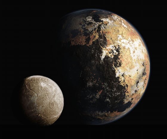
Artist's conception of Pluto's and Charon's surfaces. From http://www.ourpluto.org/home.

Artist’s conception of Pluto’s and Charon’s surfaces. From http://www.ourpluto.org/home.

We talked briefly about several things at Friday’s Journal Club. First, we discussed astrobites.org, a great blog that covers the interesting nitty-gritty of astronomy research. I pointed out that they are requesting submissions from undergrad researchers.

Second, we discussed the New Horizons mission’s request for suggestions for names of features on the surface of Pluto and its moons. After the mission flies by the system, there will be mounds of high resolution images, probably showing a variety of complex surface morphologies. And all that stuff is going to need names.

Third, Jacob presented a recent paper that extends the Titius-Bode relation to extrasolar systems and predict there are about 2 planets in habitable zones per star in our galaxy. A potentially fascinating result, but unfortunately, the T-B relation is probably just an interesting coincidence for our solar system — it has no theoretical basis, and so there’s no reason to believe it can be generalized to other planetary systems. Nevertheless, the article got a lot of press last week.

Finally, we talked about coding in astronomy, and I wanted to post this resource I just heard about, https://python4astronomers.github.io/. Looks to have a lot of helpful tutorials relevant to astronomy.

Friday’s attendees included Jennifer Briggs, Trent Garrett, Nathan Grigsby, Tanier Jaramillo, Emily Jensen, Liz Kandziolka, and Jacob Sabin.

At Friday’s journal club, we discussed on two papers. The first, Webber et al. (2015), investigated the effects of clouds on the phase curves for hot Jupiters. Webber et al. found that planet’s phase curve may depend sensitively on whether clouds are distributed uniformly or heterogenously throughout the atmosphere. They also found that the amount of light reflected by an exoplanet depends on the composition of the clouds — clouds made of rocky minerals like MgSiO3 and MgSi2O4 are much brighter than Fe clouds.

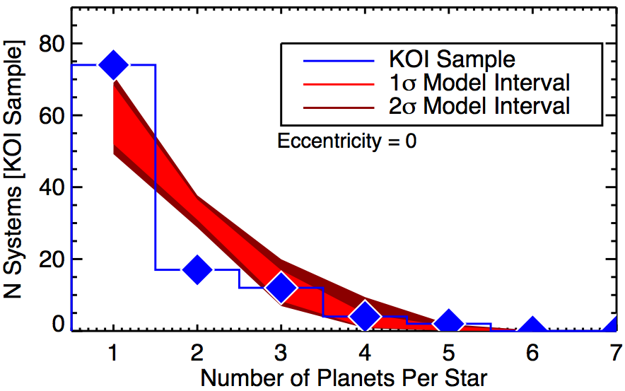
From Ballard & Johnson (2015), this figure compares the number of stars with a certain number of planets detected by Kepler (blue diamonds) to our expectations (in red) if single planet systems actually had more planets hidden from Kepler's view. The disagreement between the blue and red curves suggests that many of those apparently singleton planets really are only children and single and multi-planet systems are inherently different.

From Ballard & Johnson (2015), this figure compares the number of stars with a certain number of planets detected by Kepler (blue diamonds) to our expectations (in red) if single planet systems actually had more planets hidden from Kepler’s view. The disagreement between the blue and red curves suggests that many of those apparently singleton planets really are only children and single and multi-planet systems are inherently different.

The second paper, Ballard & Johnson (2014), investigated the frequency of exoplanets around M-dwarf stars observed by the Kepler mission. Because the Kepler mission found planets by looking for transits, there’s always a good chance that a system with only one detected planet actually has more that just don’t pass in front of their host star as seen from Earth. But we know exactly how to account for this geometric effect.

By accounting for it, Ballard and Johnson showed that Kelper actually found a lot more systems with only one planet than we would expect if there were just more planets in those systems hidden from Kepler‘s view. So there are two distinct kinds of planetary systems around M-dwarfs: those with only one planet (or possibly several planets with large mutual inclinations) and those with several.

Why the difference? Ballard and Johnson find tantalizing hints that  stars hosting only one detected planet are older on average. One simple explanation: given enough time, systems with many planets become unstable, and the lonely planets we see today originally had siblings that were gravitationally cast out of the system, to wander the void between the stars. Or the siblings were accreted by their parent stars, like Saturn eating his children. Along with many others, this study helps show that planetary systems can be much more violent places than astronomers originally thought.

Journal club attendees included Jennifer Briggs, Nathan Grigsby, Jared Hand, Tanier Jaramillo, Emily Jensen, Liz Kandziolka, and Jacob Sabin.