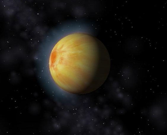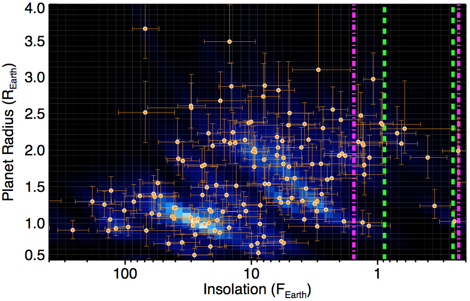
The radii of planets found in the Kepler dataset by Dressing & Charbonneau (2015) as a function of the amount of star light (insolation) they receive. The pink and green lines show ranges of insolation we think might allow the planets to be habitable.

The radii of planets found in the Kepler dataset by Dressing & Charbonneau (2015) as a function of the amount of star light (insolation) they receive. The pink and green lines show ranges of insolation we think might allow the planets to be habitable.

In journal club today, we discussed a recent study by Dressing & Charbonneau (2015) that used the Kepler dataset to search for possibly habitable planets around small (M-dwarf) stars.

Dressing and Charbonneau applied a sophisticated and comprehensive search scheme to look for habitable planets and estimate how effective their search was in finding such planets. Based on their analysis, they estimated that about 1 in 4 M-dwarf stars have planets about the size of Earth in their habitable zones and that the nearest such planet is about 8.5 light years away.

This is far enough that we’d probably still need a generation ship to reach it but a lot closer than one case, 20 light years to the nearest habitable planet, considered by Hein et al. (2012) in their analysis of interstellar colonization. This reduction in travel time could reduce the minimum population required to make the trip from maybe 7,000 to 4,000 people.

Of course, the habitable planet sought in such a trip would orbit a much cooler, redder star than the Sun, so the colonists should be prepared to plant very different crops than we have on Earth.

Attendees of today’s journal club included Simon Pintar, Nathan Grigsby, Jacob Sabin, Tyler Wade, Liz Kandziolka, Jennifer Briggs, and Emily Jensen.


Simulated dust tails around the disintegrating planet EPIC 201637175 b. From Sanchis-Ojeda+ (2015).

Simulated dust tails around the disintegrating planet EPIC 201637175 b. From Sanchis-Ojeda+ (2015).

Fun research group meeting today. We discussed research papers on a new class of extrasolar planet, ultra-short period planets. Most of these planets are small and rocky, and some of them are so small, rocky, and hot that they are actively disintegrating.

We first discussed Spitzer Space Telescope observations by Demory and colleagues of 55 Cnc e, a rocky planet with a mass and radius eight and two times the Earth’s, respectively, but almost 100 times closer to its star than the Earth is to the Sun. Its surface temperature is about 2000 K, hot enough to form a molten rock lake on the planet’s dayside.

Demory and colleagues looked at 55 Cnc e’s transits and eclipses from 2011 and 2013 and found that they changed quite a lot. Why they’ve changed isn’t clear. Demory et al. speculated that perhaps the planet exhibits extreme volcanic activity, similar to Jupiter’s moon Io, and the erupted material has gone into orbit around the star, causing variable transits and eclipses.

We next discussed the discovery of a new disintegrating rocky planet using data from the K2 mission by Sanchis-Ojeda and colleagues.

This planet, EPIC 201637175 b, zips around its star every 9 hours, and because it’s so hot (1500 K), its rocky surface is evaporating, leaving behind a dust tail, like a comet. Subtle indications of the dust tail appear in the K2 measurements as tell-tale bumps in the light curve, suggesting the dust is scattering light in complicated and surprising ways.

More follow-up work will help us understand this new extreme class of planet, perhaps even allow us to figure out what they’re made of and where they came from.

Attendees at today’s group meeting include Jennifer Briggs, Emily Jensen, Liz Kandziolka, and Tyler Wade.

From http://amzn.to/1B4bBhV.

From http://amzn.to/1B4bBhV.

Just finished Mark Essig‘s Edison and The Electric Chair. I received the book as a surprise gift, not having heard of it before. Very glad I did.

The book covers a period in American history that I knew next to nothing about — the Gilded Age and the War of the Currents. It traces Thomas Edison‘s work developing and marketing many of the key elements of the US’s electrical landscape, from the light bulb to the distribution system. Along the way, Essig weaves in elements and anecdotes from Edison’s life to paint a fascinating and nuanced picture.

Essig also describes the political landscape of Edison’s time and how social movements to reduce human and animal suffering at the turn of the last century drove the search for more humane execution methods — the most common method at the time was hanging.

Although I couldn’t put it down, I was a little disappointed by how light the book was on the scientific and technical aspects of the story. For instance, Essig spends many chapters on the public debate that raged during the War of the Currents over whether direct or alternating current was more dangerous (seems it’s AC). But he never really resolves the debate or explains our current understanding.

So it’s really more a history of science and technology than a popular science book but still a very engaging read.


As part of a project, I’m trying to learn how to do motion capture on videos. Fortunately, there’s Python support for the OpenCV computer vision library.

I adapted some motion capture code I found online that uses the Shi-Tomasi Corner Detector scheme to find good features to track — regions in a grayscale video frame that have large derivatives in two orthogonal directions.

Then the code estimates the optical flow using the Lucas-Kanade method, which applies a least-squares fit to solve for the two-dimensional velocity vector of the corner features.

As a test case, I used a video of Alice singing the “Ito Maki Maki” song.

The shiny tracks in the video show the best-fit model. Interestingly, the corner detection scheme chooses to follow the glints in her eyes and on her lip. The motion tracker does a good job following the glints until she blinks and swings her arm across her face.

The code I used is posted below.

import numpy as np
import cv2
cap = cv2.VideoCapture('IMG_0986.mov')
size = (int(cap.get(cv2.cv.CV_CAP_PROP_FRAME_WIDTH)),
int(cap.get(cv2.cv.CV_CAP_PROP_FRAME_HEIGHT)))

# params for ShiTomasi corner detection
feature_params = dict( maxCorners = 100,
qualityLevel = 0.3,
minDistance = 7,
blockSize = 7 )

# Parameters for lucas kanade optical flow
lk_params = dict( winSize = (15,15),
maxLevel = 2,
criteria = (cv2.TERM_CRITERIA_EPS | cv2.TERM_CRITERIA_COUNT, 10, 0.03))

# Create some random colors
color = np.random.randint(0,255,(100,3))

# Take first frame and find corners in it
ret, frame = cap.read()
old_gray = cv2.cvtColor(frame, cv2.COLOR_BGR2GRAY)
p0 = cv2.goodFeaturesToTrack(old_gray, mask = None, **feature_params)

# Create a mask image for drawing purposes
mask = np.zeros_like(frame)

images = list()

height , width , layers = frame.shape

fourcc = cv2.cv.CV_FOURCC('m', 'p', '4', 'v')
video = cv2.VideoWriter()
success = video.open('Alice_singing.mp4v', fourcc, 15.0, size, True)

ret = True
while(ret):
  print(ret)

  frame_gray = cv2.cvtColor(frame, cv2.COLOR_BGR2GRAY)

# calculate optical flow
  p1, st, err = cv2.calcOpticalFlowPyrLK(old_gray, frame_gray, p0, None, **lk_params)

# Select good points
  good_new = p1[st==1]
  good_old = p0[st==1]

# draw the tracks
  for i,(new,old) in enumerate(zip(good_new,good_old)):
    a,b = new.ravel()
    c,d = old.ravel()
    cv2.line(mask, (a,b),(c,d), color[i].tolist(), 2)
    cv2.circle(frame,(a,b),5,color[i].tolist(),-1)

  img = cv2.add(frame,mask)

  video.write(img)
  ret,frame = cap.read()

# Now update the previous frame and previous points
  old_gray = frame_gray.copy()
  p0 = good_new.reshape(-1,1,2)

cap.release()
video.release()
cv2.destroyAllWindows()
Artistic rendering of 51 Peg b, from http://en.wikipedia.org/wiki/51_Pegasi_b.

Artistic rendering of 51 Peg b, from http://en.wikipedia.org/wiki/51_Pegasi_b.

For the majority of exoplanets, astronomers study the planets via indirect means, by looking for their gravitational tugs on their host stars or the shadows they cast when occult their stars. Consequently, the things astronomers learn about exoplanets often involve systematic uncertainties, usually related to uncertainties about our knowledge of the stellar properties.

For example, by measuring a planet’s gravitational tugs on its star, astronomers can estimate the planet’s mass but only if they also know the star’s mass. It’s a little like watching two dancers spinning hand-in-hand, with one in black and the other in white,  and then trying to estimate the weight of the dancer in black based on how the dancer in white spins.

But in last week’s journal club, we discussed a recent study from Martins and colleagues that may have thrown white clothes on one of the most famous exoplanets, 51 Pegasi b, and revealed its dance moves.

51 Peg was the first exoplanet discovered around a Sun-like star. It’s a gas giant, like Jupiter, but unlike Jupiter, it orbits its host star every four days and is almost 100 times closer to its host star than Jupiter is to our Sun.

Martins and colleagues conducted ground-based spectroscopic observations of the 51 Peg system as the planet revolved about its host star. In principle, this orbital motion causes the spectral features imprinted on light reflected from the planet’s atmosphere to be Doppler-shifted.

Detecting the light reflected from a planet and resolving it spectrally is a bit like trying to discern the color of a football fan’s t-shirt against the glare of stadium lights, only much harder.

However, Martins and colleagues found tentative indications of light reflected from 51 Peg b’s atmosphere. By modeling the Doppler-shifting of the subtle spectral signals, they were able to estimate the planet’s mass (0.46 times Jupiter’s) and its radius (almost twice Jupiter’s, if it’s about twice as reflective as Jupiter).

Journal club attendees included Jennifer Briggs, Nathan Grigsby, Emily Jensen, and Liz Kandziolka.

With the help of physics major Jared Hand, we’ve started a weekly meeting group here in physics to discuss scientific computing — the Boise State SciComp Workshomp.

The meetings take place in the physics building, room MP408, and will focus on the nitty gritty of scientific computing — how to install and run various codes and packages.

We’ve started a github repository for the group: https://github.com/decaelus/BoiseState_SciComp_Workshomp.

We will keep a log of our meetings on the associated wiki: https://github.com/decaelus/BoiseState_SciComp_Workshomp/wiki/Working-with-Git.

We’re currently working through a presentation from the Software Carpentry Foundation on using git: http://slides.com/abostroem/local_version_control#.

At journal club today, we talked about a study from Heller and Pudritz that looks at the formation of moons around gas giant planets in extrasolar systems.

Heller and Pudritz modeled the conditions in circumplanetary disks around Jupiter-like planets to find where temperatures are right for icy moons like Jupiter’s to form. Like Goldilocks, moon formation requires conditions that are juuust right: the planet can’t be too close to its star or too small.

But given the right conditions, moons will happily accrete around a gas giant and the most massive circumplanetary disks around super-Jovian planets can form moons the size of Mars.

Heller and Pudritz point out that this means if we find an icy moon around one of the many gas giant exoplanets orbiting at about 1 AU from their host stars, we can infer the planet didn’t form there. Instead, it must have formed farther out and migrated in.

And at 1 AU around a Sun- like star, the discovery of such an exomoon would naturally make it a high priority target for habitability studies.

Attendees at today’s journal club included Nathan Grigsby, Jared Hand, Catherine Hartman, Emily Jensen, Liz Kandziolka, and Jacob Sabin.

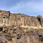
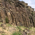
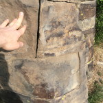
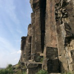
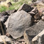
Found some beautiful basalt columns around Lucky Peak State Park just east of Boise. A quick google search doesn’t turn up any previous surveys, so these could make a good spot for some follow-on studies to our field work back in 2011.

github-octocatHad our first Scientific Computing Discussion group meeting on Friday at noon. These meetings are intended to familiarize our students with scientific computing applications and how to manage and maintain various science computing modules. We started a github repository where we’ll post notes and other information: https://github.com/decaelus/BoiseState_PAC_Workshop.

Attendees included Liz Kandziolka, Emily Jensen, Jennifer Briggs, Ahn Hyung, Tiffany Watkins, Jesus Caloca, and Helena Nikolai. Jared Hand helped lead the discussion. (Apologies to those of you who attended but I didn’t record your name.)

Had fun playing with the telescope again last night on BSU’s campus.

This time, we observed 55 Cnc, one of very few naked-eye stars that hosts transiting exoplanets. 55 Cnc’s planetary system comprises five fairly large planets, including one twice the size and eight times the mass of Earth in an orbit that roasts its surface at a temperature of 2,360 K — hot enough to vaporize iron.

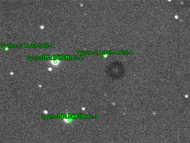
Below is our image of the sky, annotated by the astrometry.net service (try to ignore the dark doughnut that is probably a dust mote on the telescope). 55 Cnc is the bright star at the bottom and is also called HD 75732.

55 Cnc observed by BSU's campus.

55 Cnc observed by BSU’s campus.