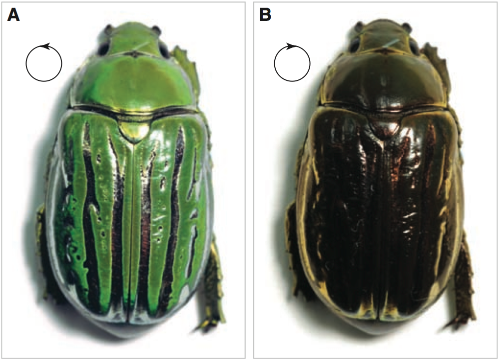
At Friday’s journal club, we discussed on two papers. The first, Webber et al. (2015), investigated the effects of clouds on the phase curves for hot Jupiters. Webber et al. found that planet’s phase curve may depend sensitively on whether clouds are distributed uniformly or heterogenously throughout the atmosphere. They also found that the amount of light reflected by an exoplanet depends on the composition of the clouds — clouds made of rocky minerals like MgSiO3 and MgSi2O4 are much brighter than Fe clouds.
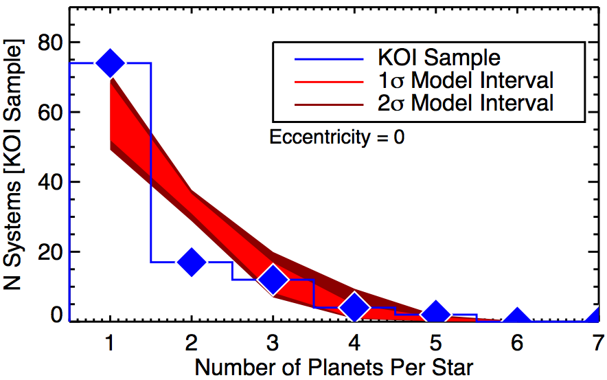
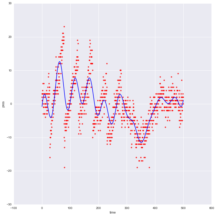
From Ballard & Johnson (2015), this figure compares the number of stars with a certain number of planets detected by Kepler (blue diamonds) to our expectations (in red) if single planet systems actually had more planets hidden from Kepler’s view. The disagreement between the blue and red curves suggests that many of those apparently singleton planets really are only children and single and multi-planet systems are inherently different.
The second paper, Ballard & Johnson (2014), investigated the frequency of exoplanets around M-dwarf stars observed by the Kepler mission. Because the Kepler mission found planets by looking for transits, there’s always a good chance that a system with only one detected planet actually has more that just don’t pass in front of their host star as seen from Earth. But we know exactly how to account for this geometric effect.
By accounting for it, Ballard and Johnson showed that Kelper actually found a lot more systems with only one planet than we would expect if there were just more planets in those systems hidden from Kepler‘s view. So there are two distinct kinds of planetary systems around M-dwarfs: those with only one planet (or possibly several planets with large mutual inclinations) and those with several.
Why the difference? Ballard and Johnson find tantalizing hints that stars hosting only one detected planet are older on average. One simple explanation: given enough time, systems with many planets become unstable, and the lonely planets we see today originally had siblings that were gravitationally cast out of the system, to wander the void between the stars. Or the siblings were accreted by their parent stars, like Saturn eating his children. Along with many others, this study helps show that planetary systems can be much more violent places than astronomers originally thought.
Journal club attendees included Jennifer Briggs, Nathan Grigsby, Jared Hand, Tanier Jaramillo, Emily Jensen, Liz Kandziolka, and Jacob Sabin.