
Simulated dust tails around the disintegrating planet EPIC 201637175 b. From Sanchis-Ojeda+ (2015).
Fun research group meeting today. We discussed research papers on a new class of extrasolar planet, ultra-short period planets. Most of these planets are small and rocky, and some of them are so small, rocky, and hot that they are actively disintegrating.
We first discussed Spitzer Space Telescope observations by Demory and colleagues of 55 Cnc e, a rocky planet with a mass and radius eight and two times the Earth’s, respectively, but almost 100 times closer to its star than the Earth is to the Sun. Its surface temperature is about 2000 K, hot enough to form a molten rock lake on the planet’s dayside.
Demory and colleagues looked at 55 Cnc e’s transits and eclipses from 2011 and 2013 and found that they changed quite a lot. Why they’ve changed isn’t clear. Demory et al. speculated that perhaps the planet exhibits extreme volcanic activity, similar to Jupiter’s moon Io, and the erupted material has gone into orbit around the star, causing variable transits and eclipses.
We next discussed the discovery of a new disintegrating rocky planet using data from the K2 mission by Sanchis-Ojeda and colleagues.
This planet, EPIC 201637175 b, zips around its star every 9 hours, and because it’s so hot (1500 K), its rocky surface is evaporating, leaving behind a dust tail, like a comet. Subtle indications of the dust tail appear in the K2 measurements as tell-tale bumps in the light curve, suggesting the dust is scattering light in complicated and surprising ways.
More follow-up work will help us understand this new extreme class of planet, perhaps even allow us to figure out what they’re made of and where they came from.
Attendees at today’s group meeting include Jennifer Briggs, Emily Jensen, Liz Kandziolka, and Tyler Wade.
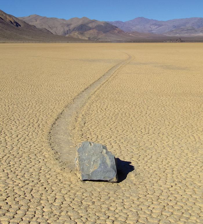 “Tucked away in California’s Death Valley National Park, the flat basin known as Racetrack Playa is littered with stones that seem to migrate across the landscape. But how do they do it? Brian Jackson describes how he and collaborators Ralph Lorenz and Richard Norris solved a long-standing mystery.” http://physicsworld.com/cws/article/indepth/2015/jul/02/the-restless-rocks-of-racetrack-playa

