 Day 1 of International Astronomical Union’s joint meeting with the American Astronomical Society in steamy Honolulu.
I attended the morning session on Dynamical astronomy in the solar system and beyond and saw some amazing talks on developments in computing planetary and satellite ephemerides, the modern day equivalent of Laplace’s Demon. These sophisticated computer programs are able to predict planetary positions to breath-taking accuracy and are sensitive enough to require including the gravitational influence of the 30 largest Trans-Neptunian Objects.
Coffee break then a late morning session on protoplanetary disks, where I learned about recent developments in the theory of disks and saw more of the beautiful disk images produced by the ALMA array.
Then a lunch session on Inclusive Astronomy led by Prof. Meredith Hughes discussing things we, as a community, can do to welcome and help people who face unusual challenges to entering and staying in the field. For example, we were advised to use sans serif fonts in our presentations because they are easier to read for those with dyslexia.
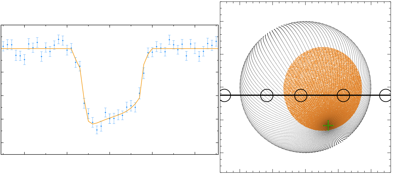
I skipped the plenary talk to attend the poster session (which were inexplicably scheduled on top of one another). I chatted with Erika Nesvold of SMACK fame about her recent result, explaining observations of an asymmetric distribution of CO in the Beta Pictoris protoplanetary disk via enhanced collisions among dust grains in the disk.
