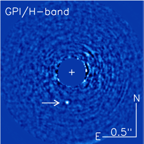
Image of 51 Eri b (indicated by arrow) in the near-infrared, 1.65 microns.
A little behind the times on this one, but we finally managed to discuss the exciting discovery of a young, Jupiter-like planet in a Jupiter-like orbit by the Gemini Planet Imager (GPI) team at journal club today.
Using high-precision optical instrumentation and some sophisticated data processing to block out the host star’s glare, the team was able to directly image the planet 51 Eri b in infrared wavelengths.
No mean feat, given that the star is more than a million times brighter than the planet and is only one ten-thousandth of a degree away in the sky. This is a little like trying to see the glow of a firefly in the end zone against the glare of a football stadium light from the 50 yard line when the two are separated by the width of a human hair*.
51 Eri b is only 20 million years old, so it’s much hotter and glows much more brightly than our own Jupiter-like planets, making it easier to see. Jupiter-like planets tend to cool in a more-or-less well-behaved way that depends partially on their masses — bigger planets start out hotter. However, the planet is much cooler than predicted by some planet formation models, which provides strong constraints on the ways in which gas giants form.
So using 51 Eri b’s estimated temperature, 700 K (400 C) and age, Macintosh et al. put its mass somewhere between 2 and 12 Jupiter masses — solidly in the planet category.
The GPI observations also show us the planet has methane and water in its atmosphere. In fact, the methane detection for this planet is the most prominent so far seen for an exoplanet, according to Macintosh.
The GPI instrument is positioned to find many more planets like this one in the coming years, so expect lots of exciting results in the next few years.
Today’s journal club attendees included Jennifer Briggs, Hari Gopalakrishnan, Tyler Gordon, and Emily Jensen.
*Macintosh et al. estimate 51 Eri b’s luminosity is about 1 millionth that of our Sun. Wikipedia indicates the star 51 Eri is about 5 times brighter than our Sun. I had a lot of trouble finding the luminosity of a firefly — this page is the best I could do, and it estimates that one firefly emits about 2 mW. Stadium lights look to emit about 1,000 W, so that gives my factor of one million in luminosity.
51 Eri b has a projected separation from its host star of 13 AU, and the star is about 96 light years away, giving an angular separation of about 2 microradians. A human hair is about 100 microns across, so it would subtend 2 microradians from a distance of about 50 yards.
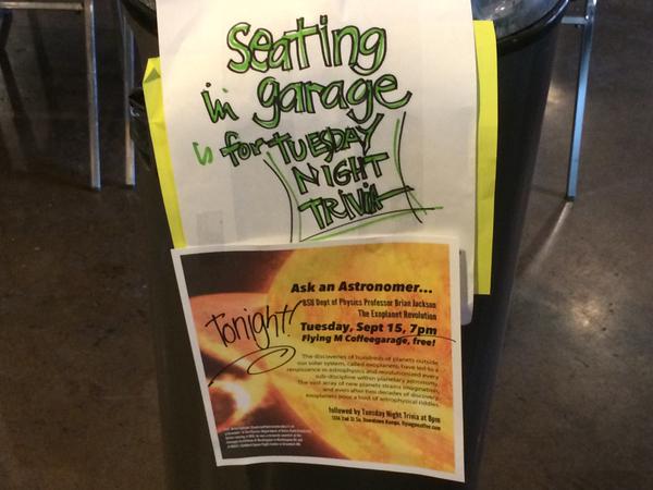
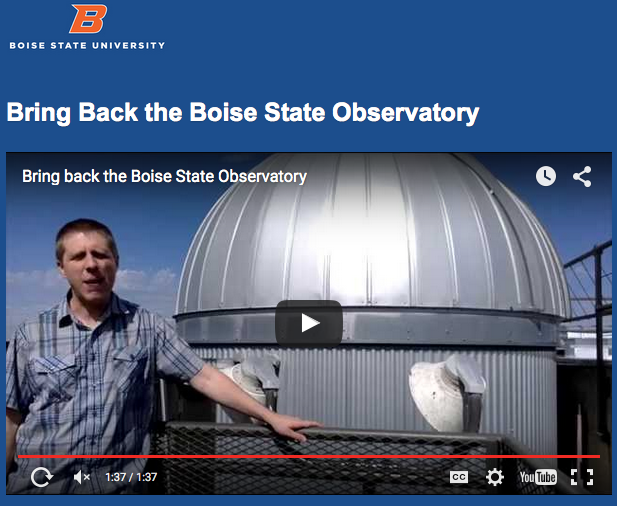
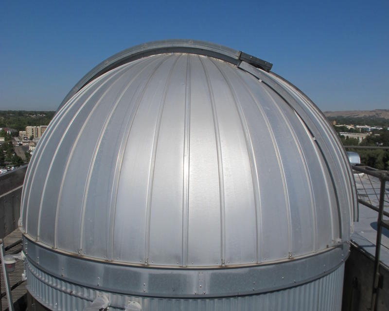
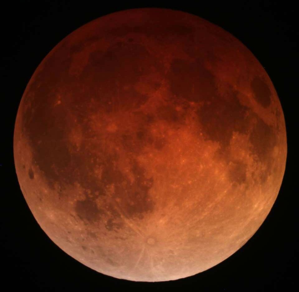 Join the Boise State Physics and Astronomy Club on the top of the Brady State Garage on Boise State’s Campus to view the last total lunar eclipse until 2018.