
A pine grove on Puget Sound’s campus.
Just recently returned from the meeting of the Northwestern Section of the American Physical Society, which took place on the lovely campus of the University of Puget Sound.
It was a cozy meeting of physicists and student physicists from throughout the northwest, and there was a variety of talks and posters on topics from gravitational waves to DNA computers to diversity in science.
One of the talks that really stuck out in my mind was the banquet presentation from Puget Sound’s Prof. James Evans about the antikythera mechanism, a mysterious barnacle-encrusted gearwork recovered from an ancient Grecian shipwreck.
Constructed by an unknown artisan in about 200 BC (according to Evans), the machine could track the date, follow lunar phases, predict solar eclipses, and even maybe show planetary motions — all with the turn of a single crank.
For my presentation, I gave a brief overview of exoplanet astronomy, with a focus on how these discoveries have begun to hone our ideas about alien life and extraterrestrial civilizations. I’ve posted by presentation below.
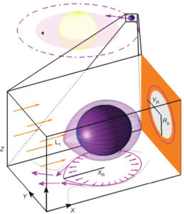
(top) WASP-12 b’s orbit. (bottom) The Roche lobe around WASP-12 b.
WASP-12 b is a planet in crisis.
One of the hottest of the hot Jupiters, the gas giant circles its Sun-like host star in a blistering 1.09-day orbit, giving its an atmosphere hot enough to vaporize rubies.
In fact, WASP-12 b is so close to its star that it very nearly fills its Roche lobe, the teardrop-shaped region inside of which material is bound to the planet. Anything on the other side of the Roche lobe falls into the gravitational clutches of the host star and can either tumble into the star or leave the system altogether.
Because WASP-12 b’s atmosphere is so hot, it is very puffy and extended, and a study from several years ago pointed out that some of the atmosphere can probably spill over the Roche lobe and escape the planet. Indeed, several groups have seen indications of outflow from WASP-12 b, meaning the planet is falling apart in front of our eyes.
Knowing what happens to the gas after escaping the planet is important for understanding the fate of the planet. If the gas goes into orbit around the star, forming an accretion disk, the planet might have billions of years before it’s destroyed. On the other hand, if the gas quickly escapes from the system or is otherwise prevented from forming a disk, the star’s gravity could rip the planet apart in an astronomical blink-of-an-eye.
A recent study from Alex Debrecht and colleagues from University of Rochester Physics and Astronomy explored what happens to gas escaping WASP-12 b. For their study, they constructed hydrodynamic models using the AstroBEAR code and found that a substantial torus of hot gas could build up around the host star in about a decade, potentially enough gas to explain the observations showing some kind of spectral absorption from the system. Such tori may commonly form in systems with ultra-hot Jupiters, so this study is probably relevant to lots of exotic exoplanets.
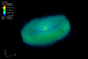
Three-dimensional simulation of gas torus in the WASP-12 system.
As interesting as these results are, though, they leave some important issues unaddressed. For instance, Debrecht and colleagues didn’t seem to include any accretion onto the host star, which might happen proceed at a fairly high rate. And the balance between outflow from the planet and accretion onto the star will go a long way to determining the amount of material in the accretion disk.
And knowing the amount of material in the disk on orbits interior and exterior to the planet’s orbit is critical for understanding the fate of WASP-12 b and other similar ultra-hot Jupiters. The accretion disk can gravitationally tug on the planet – material interior can push the planet out, while material exterior can push the planet in, potentially dooming the planet to rapid disruption.
But as is true for even the most seminal scientific work, more research is needed.
There are currently only about half a dozen Earth-sized planets orbiting stars that you can see without a telescope or binoculars, called “naked eye stars“. Among this select class, the 55 Cancri system stands out as unique – located in the constellation Cancer, 55 Cancri, a star very similar to our Sun, hosts five planets, ranging from Earth-sized to bigger than Jupiter.
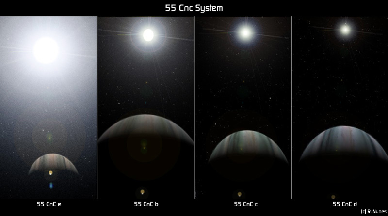
Artist’s conception of the views from four of the 55 Cancri planets. From https://en.wikipedia.org/wiki/File:55cnc.jpg.

The innermost planet, 55 Cancri e, is the one most similar to our own planet, with a mass eight times Earth’s and radius twice Earth’s.
In some big ways, though, 55 e is a far cry from Earth – it’s almost a hundred times closer to its star than we are to ours, meaning its year is only about 18 hours long. Recent observations from the Hubble Space Telescope also suggest it has a hydrogen and helium atmosphere with a pressure comparable to Earth’s. But one thing 55 e might have in common with Earth: active volcanoes.
A recent study from Patrick Tamburo of Boston University analyzed infrared observations of the 55 Cancri system collected by the Spitzer Space Telescope and found evidence for some sort of dramatic change on 55 e.
The observations were collected just as 55 e plunged behind the star as seen from the Earth. Such a configuration is referred to as a planetary eclipse or occulation.
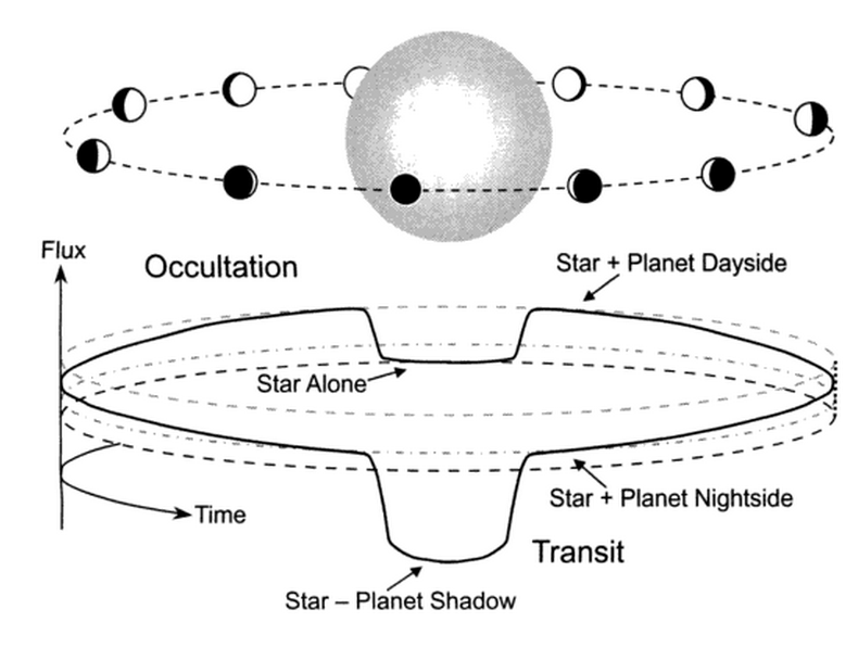
A comparison between transits and secondary eclipses (also sometimes called occultations). In a planetary transit, the planet crosses in front of the star (see lower dip) blocking a fraction of the star’s brightness. In a secondary eclipse, the planet crosses behind the star, blocking the planet’s brightness (see dip in the middle). The latter dip in brightness is fainter due to the faintness of the planet. Image credit: Josh Winn.
During an eclipse, the planet’s host star blocks out any light coming from the planet, which can produce a tiny dip in the total amount of light coming from the system.
The depth of that eclipse dip tells us how bright the dayside of the planet is – a very bright dayside would produce a big dip, indicating a hot and bright atmosphere, while a dark dayside would produce no dip, meaning a very cool atmosphere. But what if the dip is shallow during some eclipses and deep during others?
That’s exactly what Tamburo and colleagues found. In 2012, the planet exhibited eclipses with little to no depth. But when Spitzer revisited the system in 2013, it found whopping eclipses, with the planet emitting about 0.02% of the star’s light. This change corresponds to an increase in the planet’s apparent temperature of more than 1,000 degrees Kelvin (about 2,000 F).
What could cause such a dramatic change? As in the original study of these data, Tamburo and colleagues explore the possibility that an enormous volcanic eruption on 55 e could have injected dust high into the atmosphere (about 100 km up) in 2012, shrouding the lower and hotter atmosphere and surface. By 2013, the dust cloud could have settled out, raising the planet’s apparent temperature.
How plausible is this idea? Surprisingly, plausible actually. Previous studies of 55 e have shown that interactions between the planet and its sibling planets could induce enormous amounts of tidal heating within 55 e, similar to Jupiter’s moon Io, and potentially powering tremendous geophysical activity.

Eruption column rising over Redoubt Volcano, Alaska.
Large terrestrial eruptive plumes have reached 40 km height in Earth’s atmosphere, so perhaps such altitudes are not unreasonable on 55 e. However, 55 e has a surface gravity more than twice Earth’s and its atmospheric temperatures are likely much higher than Earth’s, both of which would inhibit ascent of a volcanic plume. So it’s not totally clear this exciting idea could pan out in detail.
In any case, these new results may represent the emergence a new field of study, observational exoplanetary volcanology, and maybe scientists a few generations from now will be trying to predict volcanic activity on Kilauea and Cancer.
UPDATE (2018 Jun 6) – I’m trying to learn how to use Sphinx to create documentation from source-code docstrings. The Sphinx manual is impressively opaque. Some googling turned up this document, which seems to provide useful details.
UPDATE (2018 Jun 4) – I’ve found some new resources that are much more up-to-date:
- https://jeffknupp.com/blog/2013/08/16/open-sourcing-a-python-project-the-right-way/
- Note that this article says to run the following to set up virtualenvwrapper:
echo “source /usr/local/bin/virtualenvwrapper.sh” >> ~/.zshrcHowever, that file is not located in /usr/local/bin on my Mac (High Sierra 10.13.1). Instead, I followed the instructions here to modify the command as follows:
echo “source /Users/<username>/anaconda2/bin/virtualenvwrapper.sh” >> ~/.bash_profile
- Note that this article says to run the following to set up virtualenvwrapper:
- https://cookiecutter-pypackage.readthedocs.io/en/latest/
To set up my package so it can be installed via pip, I’m following the somewhat outdated tutorial here – https://python-packaging.readthedocs.io/en/latest/index.html.
I’ll make more notes and update this post as I go along.
 As the second entry in my series on learning how to write scientific software, I’m going to describe choosing and configuring my integrated development environment or IDE. This is the program I’ll use to write and edit the source code for my project. It’s more-or-less a fancy text editor.
My text editor of choice is vim or vi improved. It’s highly customizable, powerful, and there’s lots of online help to use it. However, it has a very steep learning curve and the commands, while fast to type out, can be very cryptic. In fact, vim is famously difficult to exit.
In any case, I started using vim back when “Pirates of the Caribbean” movies were still good, so while I’m no vim guru, I feel pretty comfortable at least exiting the program.
Opening a terminal window in Mac, I fire up vim just by typing “vim” or “vi”. That opens an editor window. vim can automagically interpret and color source code, as follows:
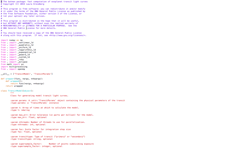
A screenshot from vim showing syntax-colored source code.
To turn on syntax coloring, go to your home directory (type “cd” in the terminal window), and edit the vim configuration file .vimrc by typing “vi .vimrc”. That should open an editor window.
Then, in vim, type the letter “i” (that starts “insert” or edit mode, allowing you to enter text into the file) and type “syntax on” <ENTER> “filetype indent plugin on”, giving a file that looks like this:

Press the escape key (which exits insert mode and enters command mode). Save the changes by typing “:wq”. That should save and exit.
Unlike many other languages, Python considers whitespace in its interpretation, and the Python style guide recommends using four spaces for each level of indentation. It would be nice to have the tab key implement that spacing in vim. Ynfortunately, my vim by default inserts eight spaces for each press of the tab key.
But you can modify that behavior by adding file-type plugin files to a special vim configuration folder. I followed the instructions here to create an ftplugin directory inside the .vim directory (by typing “cd && cd .vim && mkdir ftplugin && cd ftplugin” in the terminal window). Then, inside the directory, I created python.vim (“vi python.vim”) and again pressed “i” to enter insert mode.
I typed the following lines into the file:
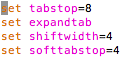
Then pressed the escape key and typed “:wq”.
Next, I tested the new configuration by typing “vi test.py” (the “.py” is important because that’s how vim knows you are editing a python file and want to use the new python configuration). I pressed tab and got four spaces instead of eight.
I’m sure there are other configuration settings that would be useful, but this’ll do for now.
UPDATE – 2018 May 17: I found this excellent website – http://docs.python-guide.org/en/latest/, which addresses vim set-up, as well as a number of other issues.
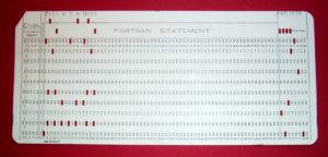
Ancient software developers meticulously punched holes in paper cards to write programs.
In the eons before my graduate career, scientists rarely, if ever, publicly distributed their codes, with authors zealously guarding their coding projects.
But just as I was finishing my PhD, it was becoming common for scientists to make the code they developed as part of a published project readily available on the internet. However, the methods to post code online (at least those I knew about) were pretty clunky.
Nowadays, the infrastructure for posting and sharing code online is robust, mature, and relatively easy to use. Consequently, scientists are creating beautiful code repositories, along with accessible documentation.
Open-sourcing code is becoming ever more important: as codes become more complex and capable, readily available codes with good documentation are critical to support reproducibility, a cornerstone of the scientific process. Moreover, federal funding agencies are starting to require investigators to make their code and data products public.
Unfortunately, since I was one of the last generation of grad students before these repositories were common, I never really learned how to distribute and document code properly.
So as part of an ongoing effort to improve my science output (and as an aide to my future students), I’m going to begin a series of semi-regular blog posts describing my process of learning how to write, document, and post scientific code.
A few caveats upfront:
- I intend to mostly (probably exclusively) write the code in python, which has become (at least in astronomy) the language of choice, so not all of what I write will be generally relevant.
- I was ushered into the Cult of Mac many years ago, so not all of what I write will be relevant for other OS’s. Here again, though, I’ve found anecdotally that most astronomers use Mac.
- This blog series is in no way intended to be comprehensive or rigorous. I’m just planning to describe what I learn as I go along, and what time I can devote will almost definitely not suffice to explain all the details, nuances, or technical aspects that intersect the project.
As to the actual science code I intend to write, several years ago my colleagues and I wrote a paper about ellipsoidal variations induced by massive exoplanets orbiting very close to their host stars. The accompanying code, EVIL-MC was written in IDL, an older language still widely used in astronomy but proprietary and requiring the purchase of an expensive site license.
My plan is to convert that IDL code into a Python package over the next several weeks.
EVIL-MC – Ellipsoidal Variations Induced by a Low-Mass Companion
Tidal distortion (exaggerated) of a star (orange-yellow disk) orbited by planet (white/black disk). The plot below shows the brightness variation of the star due to the tidal distortion.