Brian Jackson

Associate Professor of Physics at Boise State University

  • About
  • Research
    • CV
    • Joining the Boise State Planetary Science Research Group
    • Ultra-short-period planet database
    • The Short Period Planets Group — S(u)PerP(i)G
    • Google Scholar Page
    • Code
  • Teaching
  • Press
  • Extracurricular Activities
    • Field Trips
  • Public Outreach
    • Boise State’s Astronomical Observatory

Toying with Gaussian Processes

Posted by admin on February 16, 2015
Posted in: Data Science. Tagged: data science, dust devils.

Trying again to dip my toes into advanced data science, I decided to experiment with the Gaussian processes module in sci-kit learn. I’ve been working with barometric data to study dust devils, and that work involves spotting short dips in otherwise slowly varying time series.

In principle, Gaussian processes provides a way to model the slowly varying portion of the time series. Basically, such an analysis assumes the noise infesting each data point depends a little bit on the value of other nearby data points. The technical way to say this is that the covariance matrix for the data stream is non-diagonal.

So I loaded one data file into an ipython notebook and applied the sci-kit learn Gaussian processes module to model out background oscillations. Here’s the notebook.

In [32]:
%matplotlib inline
#2015 Feb 15 -- A lot of this code was adapted from 
#  http://scikit-learn.org/stable/auto_examples/gaussian_process/plot_gp_regression.html.

import numpy as np
from sklearn.gaussian_process import GaussianProcess
from matplotlib import pyplot as pl
import seaborn as sns
import pandas as pd
sns.set(palette="Set2")

#from numpy import genfromtxt

my_data = np.genfromtxt('Location-A_P28_DATA-003.CSV', delimiter=',', skip_header=7, usecols=(0, 1), names=['time', 'pressure'])

X = np.atleast_2d(np.array(my_data['time'])[0:1000]).T
y = np.atleast_2d(np.array(my_data['pressure'])[0:1000]).T
y -= np.median(y)

# Instanciate a Gaussian Process model
gp = GaussianProcess(theta0=1e-2, thetaL=abs(y[1]-y[0]), thetaU=np.std(y), nugget=1e-3)

# Fit to data using Maximum Likelihood Estimation of the parameters
gp.fit(X, y)

# Make the prediction on the meshed x-axis (ask for MSE as well)
y_pred, MSE = gp.predict(X, eval_MSE=True)
sigma = np.sqrt(MSE)

data = pd.DataFrame(dict(time=X[:,0], pres=y[:,0]))
sns.lmplot("time", "pres", data=data, color='red', fit_reg=False, size=10)

predicted_data = pd.DataFrame(dict(time=X[:,0], pres=y_pred[:,0]))
pl.plot(X, y_pred, color='blue')
Barometric time series. Pressure in hPa, and time in seconds.

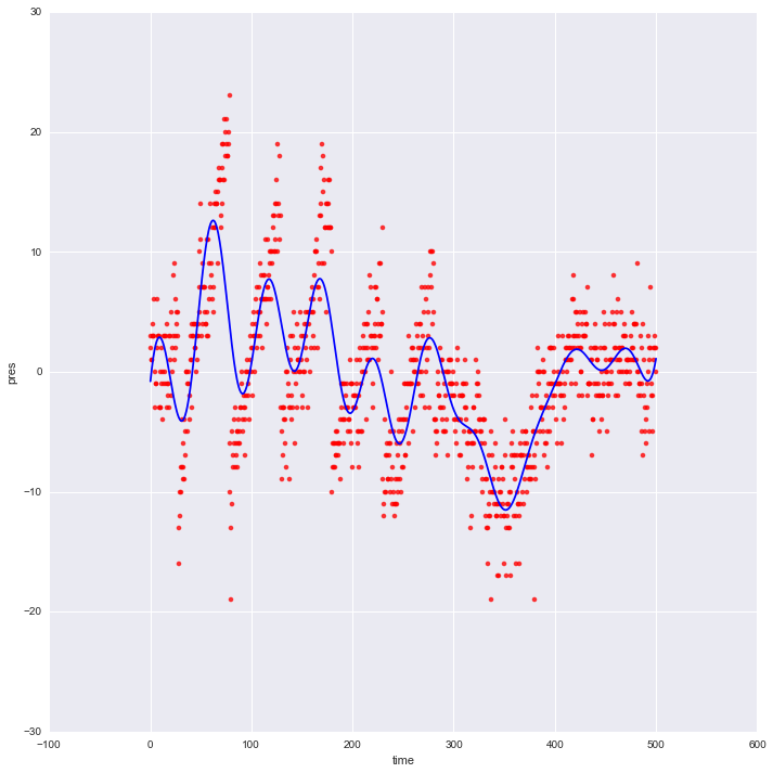
Barometric time series. Pressure in hPa, and time in seconds. The red dots show the original data, and the blue line the fit from the Gaussian process.

Unfortunately, the time series has some large jumps in it, and these are not well described by the slowly varying Gaussian process. What causes these jumps is a good question, but for the purposes of this little analysis, they are a source of trouble.

Probably need to pursue some other technique. Not to mention that the time required to perform a Gaussian process analysis scales with the third power of the number of data points, so it will get very slow very fast.

Posts navigation

← Journal Club — 2015 Feb 13
Webber+ (2015) and Ballard & Johnson (2014) →
  • Twitter: decaelus

    Brian Jackson
    • @idahoans Black Americans were not guaranteed citizenship from the nation's founding in 1776 until 1868, almost 100… https://t.co/5WA125Dj2U about 15 hours ago in reply to idahoans
    • @theidaho97 What's our play, @theidaho97? What can we do next? about 15 hours ago in reply to theidaho97
    • @ironywithab The rule in our house is just don’t say those words around grandma. about 22 hours ago in reply to ironywithab
    @decaelus
  • Recent Posts

    • Boise State Geosciences Seminar – 2021 Mar 29
    • Third Thursday Virtual Planetarium Show – 2021 Mar 18
    • First Friday Astronomy – Seeing the Dark Side of the Universe through Cosmic Lenses – 2021 Apr 2
    • Third Thursday Planetarium Show – 2021 Feb 18
    • First Friday Astronomy – Psyche: Journey to a Metallic World – 2021 Mar 5
  • Archives

    • March 2021
    • February 2021
    • January 2021
    • December 2020
    • November 2020
    • October 2020
    • September 2020
    • August 2020
    • July 2020
    • June 2020
    • May 2020
    • April 2020
    • March 2020
    • February 2020
    • January 2020
    • December 2019
    • November 2019
    • October 2019
    • September 2019
    • August 2019
    • July 2019
    • June 2019
    • May 2019
    • April 2019
    • March 2019
    • February 2019
    • January 2019
    • December 2018
    • November 2018
    • October 2018
    • September 2018
    • August 2018
    • July 2018
    • June 2018
    • May 2018
    • April 2018
    • March 2018
    • February 2018
    • January 2018
    • December 2017
    • November 2017
    • October 2017
    • September 2017
    • August 2017
    • July 2017
    • June 2017
    • May 2017
    • April 2017
    • March 2017
    • February 2017
    • January 2017
    • December 2016
    • November 2016
    • October 2016
    • September 2016
    • August 2016
    • July 2016
    • June 2016
    • May 2016
    • April 2016
    • March 2016
    • February 2016
    • January 2016
    • December 2015
    • November 2015
    • October 2015
    • September 2015
    • August 2015
    • July 2015
    • June 2015
    • May 2015
    • April 2015
    • March 2015
    • February 2015
    • January 2015
    • December 2014
    • November 2014
    • October 2014
    • September 2014
    • August 2014
    • July 2014
    • June 2014
    • May 2014
    • April 2014
    • March 2014
    • February 2014
    • January 2014
    • December 2013
    • November 2013
    • October 2013
    • September 2013
    • August 2013
    • July 2013
Proudly powered by WordPress Theme: Parament by Automattic.