Artist's conception of Pluto's and Charon's surfaces. From http://www.ourpluto.org/home.

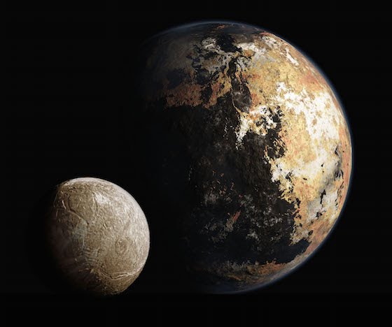
Artist’s conception of Pluto’s and Charon’s surfaces. From http://www.ourpluto.org/home.

We talked briefly about several things at Friday’s Journal Club. First, we discussed astrobites.org, a great blog that covers the interesting nitty-gritty of astronomy research. I pointed out that they are requesting submissions from undergrad researchers.

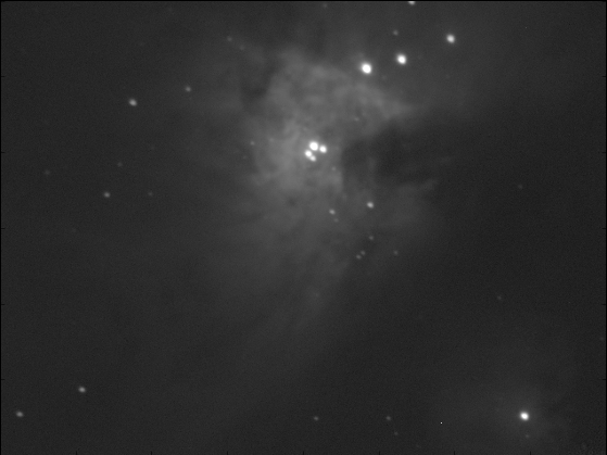
Second, we discussed the New Horizons mission’s request for suggestions for names of features on the surface of Pluto and its moons. After the mission flies by the system, there will be mounds of high resolution images, probably showing a variety of complex surface morphologies. And all that stuff is going to need names.

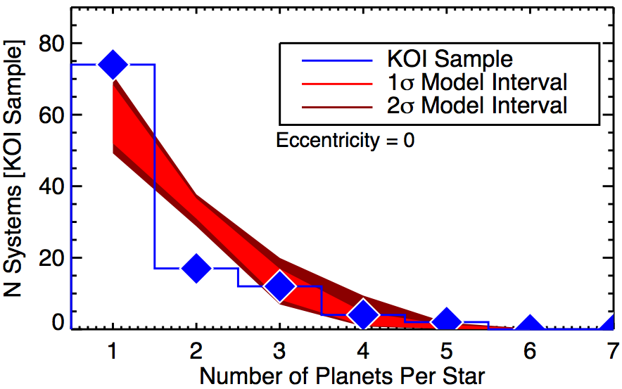
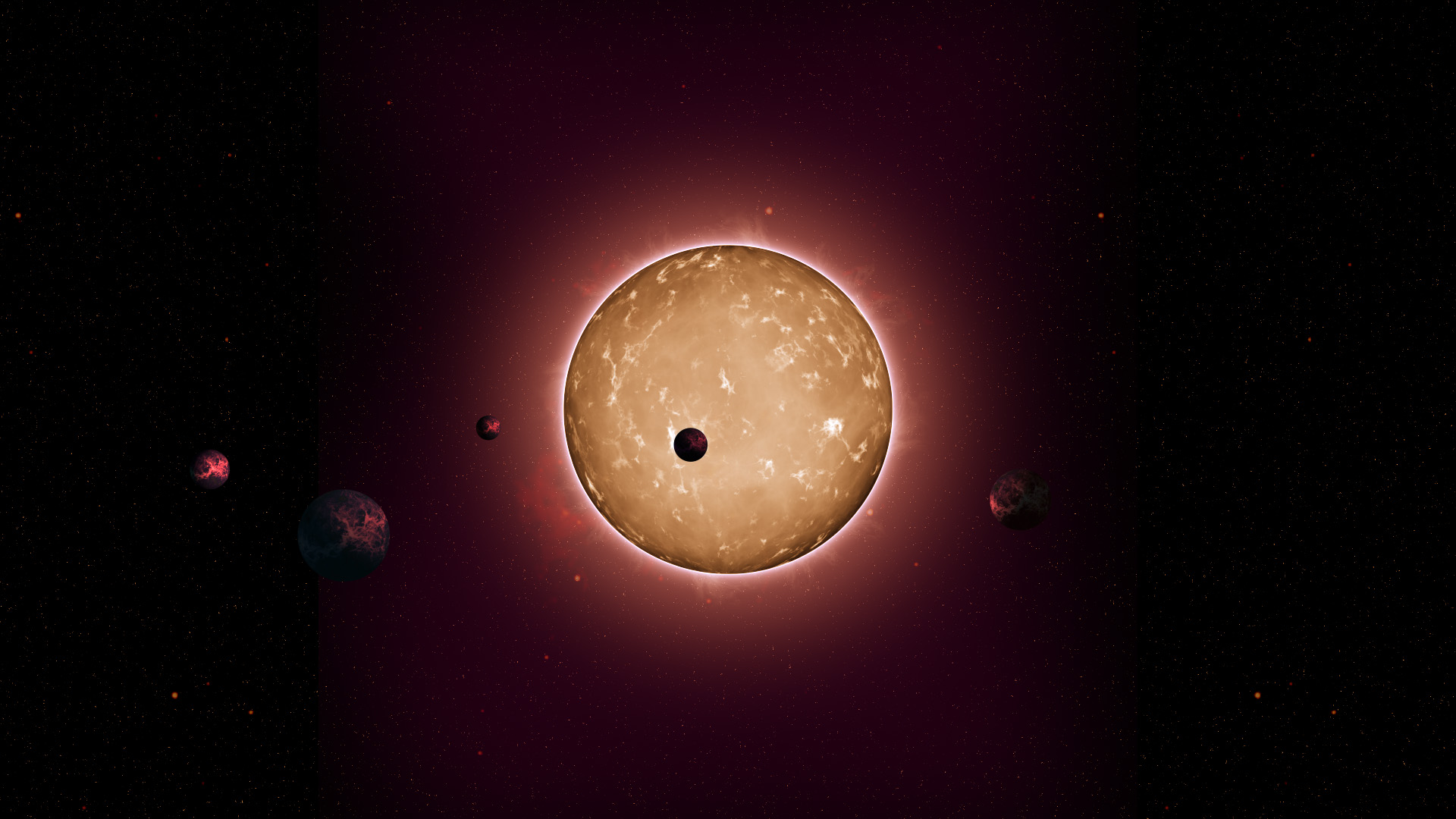
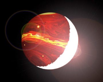
Third, Jacob presented a recent paper that extends the Titius-Bode relation to extrasolar systems and predict there are about 2 planets in habitable zones per star in our galaxy. A potentially fascinating result, but unfortunately, the T-B relation is probably just an interesting coincidence for our solar system — it has no theoretical basis, and so there’s no reason to believe it can be generalized to other planetary systems. Nevertheless, the article got a lot of press last week.

Finally, we talked about coding in astronomy, and I wanted to post this resource I just heard about, https://python4astronomers.github.io/. Looks to have a lot of helpful tutorials relevant to astronomy.

Friday’s attendees included Jennifer Briggs, Trent Garrett, Nathan Grigsby, Tanier Jaramillo, Emily Jensen, Liz Kandziolka, and Jacob Sabin.

Thanks to two of our folks in BSU physics, we’ve finally managed to get one of our telescopes working and took a beautiful image last night of the Orion Nebula.

Orion Nebula captured on-campus at Boise State on 2015 Mar 18.

Orion Nebula captured on-campus at Boise State on 2015 Mar 18.

Update (2015 Mar 29) — I submitted the FITS file image of the Orion nebula to astrometry.net, and it returned the following annotated image:

Astrometry.net fit for our Orion image. From http://nova.astrometry.net/user_images/622647#annotated.

Astrometry.net fit for our Orion image. From http://nova.astrometry.net/user_images/622647#annotated.

Just for my info, the reported image size is 14.6 x 10.9 arcmin and pixel scale is 0.547 arcsec/pixel.

Another attempt at using Gaussian processes to model time series, I’m looking at light curves from active galactic nuclei (AGN). The key thing I’m trying to do here is find and model flaring events.

First, I was interested to see if I could spot outliers representing the peaks of flares, while using a Gaussian processes (GP) model for background variability. The document below shows that attempt. The red band in each plot shows the GP prediction if there were no significant outliers, while the red dots show the outliers. (BTW, the way I embedded the code is very klunky but explained here.)

[gview file=”http://www.astrojack.com/wp-content/uploads/2015/03/looking_for_outliers.pdf”]

Next, I wanted to try to fit one of the apparent flaring events with a model that allowed for correlated noise. To that end, I adapted the example from Foreman-Mackey’s george python module. My solution is shown below. I need to incorporate a variable number of flaring events (I only allowed one for this example), but the model fit worked pretty well. In the second plot below, the blue band shows the range of model fits from the Markov-Chain Monte-Carlo (MCMC) analysis.

[gview file=”http://www.astrojack.com/wp-content/uploads/2015/03/fit_using_GP.pdf”]

At Friday’s journal club, we discussed on two papers. The first, Webber et al. (2015), investigated the effects of clouds on the phase curves for hot Jupiters. Webber et al. found that planet’s phase curve may depend sensitively on whether clouds are distributed uniformly or heterogenously throughout the atmosphere. They also found that the amount of light reflected by an exoplanet depends on the composition of the clouds — clouds made of rocky minerals like MgSiO3 and MgSi2O4 are much brighter than Fe clouds.

From Ballard & Johnson (2015), this figure compares the number of stars with a certain number of planets detected by Kepler (blue diamonds) to our expectations (in red) if single planet systems actually had more planets hidden from Kepler's view. The disagreement between the blue and red curves suggests that many of those apparently singleton planets really are only children and single and multi-planet systems are inherently different.

From Ballard & Johnson (2015), this figure compares the number of stars with a certain number of planets detected by Kepler (blue diamonds) to our expectations (in red) if single planet systems actually had more planets hidden from Kepler’s view. The disagreement between the blue and red curves suggests that many of those apparently singleton planets really are only children and single and multi-planet systems are inherently different.

The second paper, Ballard & Johnson (2014), investigated the frequency of exoplanets around M-dwarf stars observed by the Kepler mission. Because the Kepler mission found planets by looking for transits, there’s always a good chance that a system with only one detected planet actually has more that just don’t pass in front of their host star as seen from Earth. But we know exactly how to account for this geometric effect.

By accounting for it, Ballard and Johnson showed that Kelper actually found a lot more systems with only one planet than we would expect if there were just more planets in those systems hidden from Kepler‘s view. So there are two distinct kinds of planetary systems around M-dwarfs: those with only one planet (or possibly several planets with large mutual inclinations) and those with several.

Why the difference? Ballard and Johnson find tantalizing hints that  stars hosting only one detected planet are older on average. One simple explanation: given enough time, systems with many planets become unstable, and the lonely planets we see today originally had siblings that were gravitationally cast out of the system, to wander the void between the stars. Or the siblings were accreted by their parent stars, like Saturn eating his children. Along with many others, this study helps show that planetary systems can be much more violent places than astronomers originally thought.

Journal club attendees included Jennifer Briggs, Nathan Grigsby, Jared Hand, Tanier Jaramillo, Emily Jensen, Liz Kandziolka, and Jacob Sabin.

Trying again to dip my toes into advanced data science, I decided to experiment with the Gaussian processes module in sci-kit learn. I’ve been working with barometric data to study dust devils, and that work involves spotting short dips in otherwise slowly varying time series.

In principle, Gaussian processes provides a way to model the slowly varying portion of the time series. Basically, such an analysis assumes the noise infesting each data point depends a little bit on the value of other nearby data points. The technical way to say this is that the covariance matrix for the data stream is non-diagonal.

So I loaded one data file into an ipython notebook and applied the sci-kit learn Gaussian processes module to model out background oscillations. Here’s the notebook.

In [32]:
%matplotlib inline
#2015 Feb 15 -- A lot of this code was adapted from 
#  http://scikit-learn.org/stable/auto_examples/gaussian_process/plot_gp_regression.html.

import numpy as np
from sklearn.gaussian_process import GaussianProcess
from matplotlib import pyplot as pl
import seaborn as sns
import pandas as pd
sns.set(palette="Set2")

#from numpy import genfromtxt

my_data = np.genfromtxt('Location-A_P28_DATA-003.CSV', delimiter=',', skip_header=7, usecols=(0, 1), names=['time', 'pressure'])

X = np.atleast_2d(np.array(my_data['time'])[0:1000]).T
y = np.atleast_2d(np.array(my_data['pressure'])[0:1000]).T
y -= np.median(y)

# Instanciate a Gaussian Process model
gp = GaussianProcess(theta0=1e-2, thetaL=abs(y[1]-y[0]), thetaU=np.std(y), nugget=1e-3)

# Fit to data using Maximum Likelihood Estimation of the parameters
gp.fit(X, y)

# Make the prediction on the meshed x-axis (ask for MSE as well)
y_pred, MSE = gp.predict(X, eval_MSE=True)
sigma = np.sqrt(MSE)

data = pd.DataFrame(dict(time=X[:,0], pres=y[:,0]))
sns.lmplot("time", "pres", data=data, color='red', fit_reg=False, size=10)

predicted_data = pd.DataFrame(dict(time=X[:,0], pres=y_pred[:,0]))
pl.plot(X, y_pred, color='blue')
Barometric time series. Pressure in hPa, and time in seconds.

Barometric time series. Pressure in hPa, and time in seconds. The red dots show the original data, and the blue line the fit from the Gaussian process.

Unfortunately, the time series has some large jumps in it, and these are not well described by the slowly varying Gaussian process. What causes these jumps is a good question, but for the purposes of this little analysis, they are a source of trouble.

Probably need to pursue some other technique. Not to mention that the time required to perform a Gaussian process analysis scales with the third power of the number of data points, so it will get very slow very fast.

We had an abbreviated meeting, as everyone (including myself) seems to have been unusually busy this week. No specific research updates, but we discussed two interesting articles of science news. Attendees were Liz Kandziolka, Jennifer Briggs, Emily Jensen, Brenton Peck, Nathan Grigsby, Trent Garrett, and Prof. Daryl Macomb.

The first article we discussed, “Cosmology from Quantum Potential“, proposed an origin for the universe that represents an alternative to the big bang. We didn’t really understand the theory, but it seems to involve the idea that universe doesn’t really have a beginning. We puzzled over whether the theory actually proposes any specific testables or observables.

The second article we discussed, “Titan Submarine : Vehicle Design and Operations Concept for the Exploration of the Hydrocarbon Seas of Saturn’s Giant Moon“, suggests a plan to send a submersible to plumb the depths of Titan’s seas, the only seas in our solar system besides those on Earth. Studying Titan’s seas may teach us about the pre-biotic chemistry in the Earth’s early oceans. And as with all exciting scientific work, this study comes with an animation and dramatic sound track.

The tightly packed system, named Kepler-444, is home to five small planets in very compact orbits. The planets were detected from the dimming that occurs when they transit the disc of their parent star, as shown in this artist's conception. From http://www.nasa.gov/ames/kepler/astronomers-discover-ancient-system-with-five-small-planets/.

The tightly packed system, named Kepler-444, is home to five small planets in very compact orbits. The planets were detected from the dimming that occurs when they transit the disc of their parent star, as shown in this artist’s conception. From http://www.nasa.gov/ames/kepler/astronomers-discover-ancient-system-with-five-small-planets/.

In journal club on Friday, we discussed a fascinating paper from Campante and colleagues announcing discovery of one of the oldest planetary systems ever discovered — Kepler-444. The system comprises five planets, ranging from roughly Mercury- to Venus-sized with orbital periods from about 3 to 9 days.

Studying the frequencies of oscillations within the K-dwarf host star (an approach known as asteroseismology), Campante et al. estimate the host star, and therefore probably the planets, is about 11 billion years old, almost as old as the Milky Way galaxy itself.

To put that age into perspective, by the time our solar system formed, about 5 billion years ago, the Kepler-444 was already a billion years older than our solar system is now.

The existence of such an old system tells us that rocky planets began forming almost as soon as the Milky Way itself formed, which allows for the exciting possibility of very ancient life in the galaxy.

Present at journal club were Jennifer Briggs, Trent Garrett, Nathan Grisgby, Emily Jensen, Liz Kandziolka, Brenton Peck, and Jacob Sabin.

Pressure variations (in hectoPascal, hPa) vs. local time for one dust devil pressure dip. The blue curve shows our model fit.

Pressure variations (in hectoPascal, hPa) vs. local time for one dust devil pressure dip. The blue curve shows our model fit.

Dust devils occur in arid climates on the Earth and ubiquitously on Mars. Martian dust devils have been studied with orbiting and landed spacecraft, while most studies of terrestrial dust devils have involved manned monitoring of field sites, which can be costly both in time and personnel. As an alternative approach, my colleague Ralph Lorenz and I performed a multi-year in-situ survey of terrestrial dust devils using pressure loggers deployed at El Dorado Playa in Nevada, USA, a site known for dust devil activity.

When a dust devil passed over our pressure sensors, it appeared as a pressure dip in the time series, as illustrated in the figure. By modeling these signals, we learned a lot of about dust devils. For instance, in spite of expectations, we found signals that looked a lot like dust devils that occurred at night and even in the winter. So do dust devils happen year-round, day and night? More work will help us figure it out.

Our paper on this study will appear soon in the Journal of Geophysical Research Planets.

From https://emps.exeter.ac.uk/physics-astronomy/research/astrophysics/phd-opportunities/modelling-shock-waves/.

From https://emps.exeter.ac.uk/physics-astronomy/research/astrophysics/phd-opportunities/modelling-shock-waves/.

On Friday, everyone in our research group gave a little update on what they’ve been up to.

Liz and Jennifer talked about Parmentier et al.’s (2013) paper on the meteorology of hot Jupiters and how condensates are transported throughout these dynamic atmospheres.

Emily talked about working through the first few chapters of Murray & Dermott’s classic Solar System Dynamics. She will eventually study the orbital dynamics of systems of exoplanets very close to their host stars.

Brenton discussed his reading of Balme & Greeley (2006) on dust devils in preparation for working with me on terrestrial and Martian dust devils. A very exciting possibility, Brenton and the rest of the group said dust devils are common just south of Boise. Good chance we can do some in-situ monitoring locally.

Nathan spoke briefly about looking for more very short-period planets using data from the Kepler and K2 missions.

In attendance were Liz Kandziolka, Jennifer Briggs, Emily Jensen, Brenton Peck, Nathan Grigsby, Trent Garrett, and Tiffany Watkins.

Mechanical failures interrupted Kepler's original mission, but the telescope is still hunting exoplanets. From http://www.nature.com/news/three-super-earth-exoplanets-seen-orbiting-nearby-star-1.16740.

Mechanical failures interrupted Kepler’s original mission, but the telescope is still hunting exoplanets. From http://www.nature.com/news/three-super-earth-exoplanets-seen-orbiting-nearby-star-1.16740.

Discussed a brilliant paper today in journal club from Ian Crossfield and collaborators, in which they announce the discovery of a three-planet system around a nearby M-dwarf star.

The team found the new system in data from the re-incarnated Kepler mission called K2. This system is only the second discovered by the mission (the first was announced a few months ago).

This new system is especially exciting because, as the authors point out, it is observable by other available facilities, allowing astronomers to characterize the planets and star in detail.

The outermost planet in the system, with an orbital period of 45 days, is very near the inner edge of the system’s habitable zone and has a temperature of about 310 K (100 F), making it plausibly habitable. Combined with the fact that we can probably characterize the planet in detail, there’ll probably be a flurry of exciting studies of the system very soon.

Journal club was attended by Jennifer Briggs, Trent Garrett, Nathan Grigsby, Emily Jensen, Liz Kandziolka, and Brenton Peck.