Uncategorized

Artist’s conception of a hot Jupiter shedding mass.
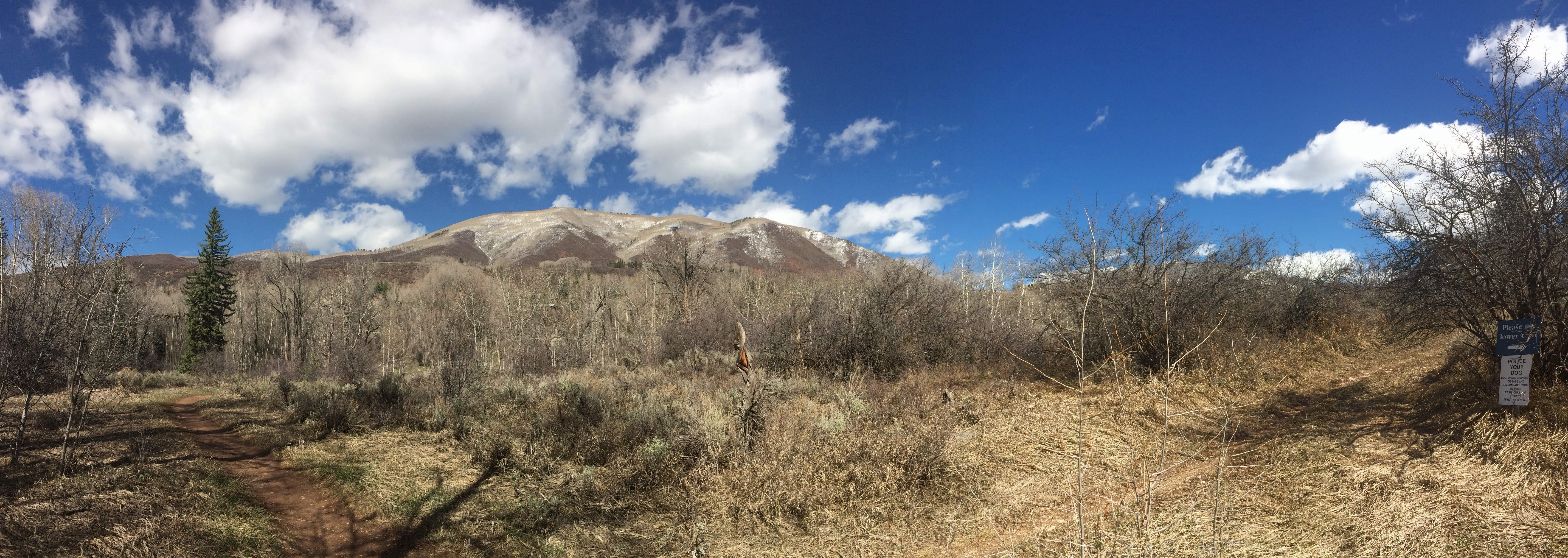
I just arrived home after a week-long visit to Aspen, CO to attend the Formation and Dynamical Evolution of Exoplanets Conference at the Aspen Center for Physics.
This conference was a cozy affair, with just over 100 attendees, and was narrowly focused on dynamical questions and approaches related to the origins and fates of exoplanet systems.
Researchers from around the world gave presentations on topics ranging from the dynamics of debris disks to observations of planet-hosting binary star systems. Blocks of presentations were punctuated by lengthy coffee breaks, when the real scientific give-and-take takes place. These interludes often give rise to groundbreaking, thesis-motivating, all-nighter-pulling research ideas.
Most of the presentations and conversations were excellent and inspiring, and I can’t do them all justice in a short blog post. So I’ll just talk about one that struck me in particular.
On Tuesday, Hanno Rein at Toronto spoke about a new N-body integrator his team has been developing in recent years, called REBOUND. This new framework may spur a revolution in dynamical modeling of astrophysical systems.
In astronomy, “n-body integration” is jargon for the numerical simulation of interactions among multiple (“n” of them) gravitating bodies. For hundreds of years, astronomers have been able to describe the orbital of two gravitating bodies quite easily, thanks to Johannes Kepler.
But as soon as you add another body to the system, there is no exact way to solve for the orbital motion of the bodies (except in very specific and limited circumstances). Even in the case of two bodies, if you want to include more complicated forces than simple gravity, solving for the orbital motion can be quite difficult.
To surmount these difficulties, scientists have turned to computer simulations to model in an approximate way the evolution of n-body systems. Although scientists have spent decades coming up with better and better models and algorithms, n-body simulations can still take a lot of computing power, and the often complicated codes can be cumbersome to set up and run. More than that, it’s often difficult or impossible for scientists to share results because there’s no good agreed-upon format for simulation output.
Rein’s REBOUND open-source code solves several of these problems at once: it employs latest modeling schemes to track orbital motions and gravitational interactions; it can be run using inside of an iPython Notebook; and it provides a uniform format for simulation output which anyone can use to re-run or re-analyze another scientists work – critical for scientific reproducibility. The iPython Notebook also provides a really neat visualization capability so you can directly watch the evolution of your astronomical system.
Time evolution of the orbits of stars in Leela’s constellation.
The code is so easy to run, in fact, that I installed and began running it immediately after Rein’s presentation. And all of its capabilities allowed me to finally simulate and visualize the evolution of a system I’ve wanted to look at for a long time – see animation at left (see here for how I created it).
I also gave a presentation on our group’s work looking at disruption of gaseous exoplanets.
And so, the combination of beautiful scenery and beautiful science made the Aspen Exoplanets conference one of the best in recent memory.
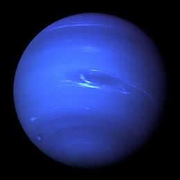
The Kepler/K2 Mission has revolutionized astronomy, having more than decupled the number of known and suspected exoplanets in just the last few years. Although we can extrapolate things we’ve learned from these distant planets to infer things about our own solar system, data from the mission have not impacted directly on our understanding of the solar system because the mission has not observed solar system objects, until now. For a recent paper, Jason Rowe and colleagues collected K2 observations of Neptune to look for the signatures of global oscillations in the planet.
What does that mean? All planets and stars exhibit intrinsic oscillations as seismic waves permeate their interiors – essentially they are ringing like giant celestial bells. On the Earth, detailed studies of these seismic waves have taught us loads about Earth’s interior, and the soon-to-launch Insight Mission will do much the same for Mars. We also study the Sun’s interior this way because we can watch as waves that originate deep within the Sun bounce around on the surface. For the Sun, these waves cause tiny oscillations in brightness every few minutes.
In the last decades, a lot of work has gone into looking for such oscillations for in gas and ice giants in our solar system, but aside from very cool indirect signatures in the rings of Saturn, no one has clearly detected global oscillations in the giant planets. Using the Kepler spacecraft, Rowe and colleagues set out to detect global oscillations by watching Neptune for 80 days. Unfortunately, in spite of a tremendous effort, they did not detect any clear oscillations from Neptune.
But amazingly, they were able to detect variations in brightness due to the Sun’s global oscillations. This is a little like seeing someone signaling with a flashlight by looking at a mirror in which the light is being reflected, only with the flashlight and mirror 4 billion kilometers apart.
The movie below shows the Kepler observations of Neptune as the planet meandered across the field of view. Keep in mind that the solar oscillations are VERY small, and the oscillations in brightness apparent in the movie are due to Neptune’s motion in the field, NOT due to the Sun. To see those oscillations, you’d need to be a computer.

It’s been miserably cold in Boise, and we’ve had record snowfall during the last few weeks.
Sunday, however, it was relatively warm — warm enough, in fact, that the snow that was slated to fall fell as sleet instead.
So I took my daughter over to a friend’s house for a playdate, and as we walked over, we heard the beautiful sound of the tiny icy pebbles clattering to the ground. The sound was so distinctive and regular that I whipped out my phone to record it.
When I got home later, it seemed like there must be something interesting I could do with the recording, and the first thing that struck me was to analyze the frequency of the clattering sound. In other words, how often did I hear a sleet pellet strike the ground?
To begin, I imported the m4a file from my iphone and then convert it via command-line into a wav file (since I planned to use python and it was easier to find ways to manipulate wav than m4a files):
ffmpeg -i Sleet_Falling.m4a Sleet_Falling.wav
Then I fired up ipython notebook and imported and plotted the wav file:
[codesyntax lang=”python”]
%matplotlib inline

import numpy as np
import wave
import matplotlib.pyplot as plt

from scipy.io import wavfile
# Load the data and calculate the time of each sample
samplerate, data = wavfile.read('Sleet_Falling.wav')
times = np.arange(len(data))/float(samplerate)

# Make the plot
# You can tweak the figsize (width, height) in inches
fig = plt.figure(figsize=(6, 4))
ax = fig.add_subplot(111)
ax.plot(times, data, lw=0.5)
ax.set_xlim([0,10])
ax.set_ylim([-2000,2000])
ax.set_xlabel('time (s)')

fig.savefig('Sleet_Falling.png', dpi=500
[/codesyntax]
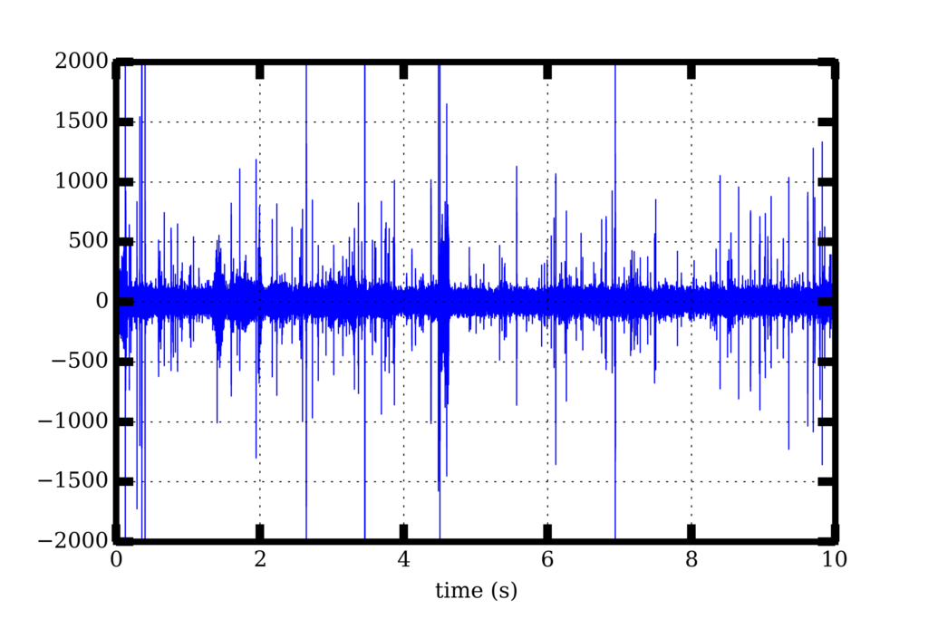
The distinctive rapid crackling is apparent in the waveform.
Next, I calculated a Fourier transform of the signal:
[codesyntax lang=”python”]
from numpy.fft import rfft

ft = np.fft.rfft(data)
n = data.size
timestep = 1./samplerate
freq = np.fft.rfftfreq(n, d=timestep)
period = 1./freq

fig = plt.figure(figsize=(6, 6))
ax = fig.add_subplot(111)
ax.semilogx(period, abs(ft), lw=0.5)

mx_arg = abs(ft).argmax()
print(period[mx_arg])

fig.savefig('Sleet_Falling_fft.png', dpi=500)
[/codesyntax]
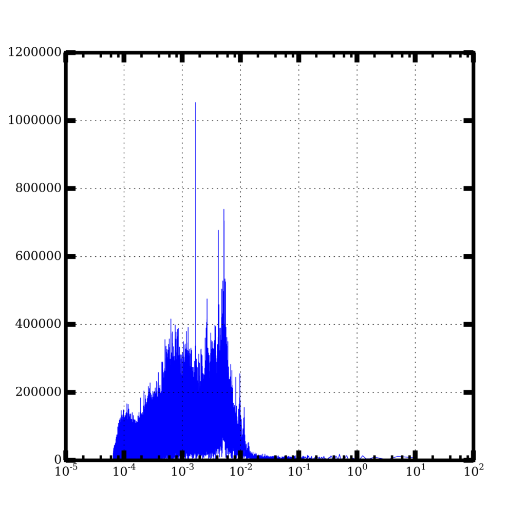
which shows a distinct peak at about 1 millisecond.
Assuming the sleet I saw is about 5 mm in radius, I estimate a terminal velocity of about 5 m/s. If I imagine (unrealistically) that the sleet particles are falling in a single column, with one directly above another and traveling at 5 m/s, then one striking the ground every millisecond means the sleet balls are basically packed end to end, as tightly as they can be [1 ms = (5 mm)/(5 m/s)]. Of course, if the pellets were spread out and striking the ground at random places, they could be way more spread out and not as many would have to fall at a time in order to make the sound I heard.
Turns out I’m not the first person to try estimating the precipitation rate using sound. NASA deploys microphones in the ocean to record the distinctive sound of raindrops.
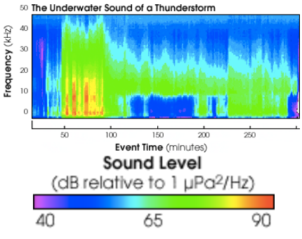
From http://earthobservatory.nasa.gov/Features/Rain/rain_2.php.
In fact, different size raindrops make different sounds because some sizes of drops generate bubbles and others do not, and so scientists can actually estimate the sizes of raindrops by just looking at the distribution of frequencies.
Unfortunately, I can’t make the same kinds of measurements using my iPhone because I haven’t calibrated the microphone using a sound of known amplitude. Maybe something for the future.
